Tuesday, July 31, 2012

FEDFUNDS and TB3MS


The Federal Funds rate is useful sometimes. But FRED's FEDFUNDS numbers go back only to the mid-1950s. So sometimes I will want to use FRED's TB3MS -- "3-Month Treasury Bill: Secondary Market Rate" -- as a proxy for FEDFUNDS.

TB3MS goes back to the mid-1930s.

Monday, July 30, 2012

How does the economy work?


That's really the question, isn't it? How does the economy work?

At The Grumpy Economist, John Cochrane (looks like Anthony DiNozzo) writes a post called Myths and Facts About the Gold Standard. The post is about doing something like the gold standard: targeting the price level.

I don't care. Me and "Grumpy" may be the only two people left in the world who would be happy with price stability. But that's a result, you know, like GDP is a result. When economists forget how the economy works, there gets to be a lot of mistaking goals for policies: We want price stability? Well, let's target price stability! We want a smoothly expanding NGDP? Well, lets target the NGDP level!

No. You guys have to throw away everything you know -- all the nonsense that got us to the crisis you couldn't see coming -- and start with something simple.

Always keep in mind the ratio between inside money and outside money.

"Imagine a government with $15 trillion of debt," Cochrane writes. Yeh, okay. But also imagine $60 trillion of private-sector debt.

Now, imagine $6 trillion instead. The burden is gone.

It is not only government debt that matters. The level of private debt matters even more. And the balance between the two is what matters most. It is the most important thing, and the most neglected.


A gold standard cannot work if it fails to manage the balance between public and private debt -- to manage, and to prevent imbalances from arising.

Price-level targeting cannot work if it fails to prevent imbalances from arising between public and private debt.

NGDP-level targeting cannot work if it fails to prevent imbalances from arising between public and private debt.

Nothing will work, that fails to prevent imbalances from arising between public and private debt -- between internal and external money, if you prefer to say it that way.

How does the economy work? It runs on money.

Cullen Roche: "the recent period of lax lending and unusual optimism"


From Pragmatic Capitalism: Failing to Connect the Boom to the Bust. Cullen Roche writes:
Since bank issued “inside money” is the primary form of money used in our fiat monetary system it’s totally normal and expected that a boom would result in credit expansions. As you can see in the chart below the rates of change in total liabilities tend to boom and bust with the business cycle. And this shouldn’t be at all surprising. When the economy booms people borrow more as they do more business, take more risk, etc. And when the boom slows and turns into a bust the credit cycle flips and the downturn ensues. Like food, we need credit expansions. But it’s when the credit cycle gets abused that we see the biggest booms and busts.


The bottom line to me is, you can’t even begin to understand the current economic machine without understanding this basic fact – we live in a fiat monetary system in which bank issued “inside money” is the primary form of money. Access to credit can exacerbate the boom as we just saw during the recent period of lax lending and unusual optimism. And the more credit the more potential for a boom (and a bust). So I wouldn’t say that rising debt levels always cause recessions, but rising debt levels certainly make it easier for economic agents to act irrationally and irresponsibly thereby substantially increasing the odds of a boom and a bust.

Number one, I like the graph. It reminds me of what I was highlighting here.

Number two, Cullen says: "bank issued 'inside money' is the primary form of money used in our fiat monetary system". Says it twice. The implication being that there is a "secondary" form of money that is "outside" money. Okay, so always keep in mind the ratio between inside money and outside money.

Here, let's think 1800s because it's easy to see gold. These days "outside" money comes from the government and it's made of nothing more substantial than paper, and it's hard to tell apart from "inside money". It's hard to tell apart. The difference is the cost of inside money, the interest cost. But that cost does not travel with the money. It stays with the borrower. So inside money looks like outside money, and debt looks like a separate problem.

But think back to a time when we didn't have the Federal Reserve, a time when we used gold for money. A time when gold prospectors performed the service that is now performed by the Fed: supplying the economy with outside money.

In cowboy movies, the prospector always walks into the saloon with his bag of gold. It's good for the movies. In real life, more likely the prospector walked into the mint and had his gold made into coins and he spent the coins, and that was how outside money came into the economy. Anyway, somebody had it coined.

Or people would leave their gold at the goldsmith's, or at the bank, and get receipts for it. And they would use the receipts to buy things. And the goldsmith, or the bank, might lend out the gold to a borrower. The bank might even put the gold in the borrower's "account" and give the borrower paperwork in stead of gold. And the borrower might spend that paper.

And if you stop and look at that, the paper that the depositor spends is inside money -- money created within the economy, not brought to it by a prospector -- and the paper that the borrower spends is inside money, and there is now more paper money than gold.

We don't use gold like that anymore. And that makes it hard to see the difference between inside money and outside money. But the main difference is the cost of it. The cost of it is the interest cost, plus the payback. And you can get a feel for that cost by looking at debt today.

And you can get a feel for outside money by looking at the money for which there is no such cost. Like the money that people have, which is the money in circulation, or M1 money.

And you can get a feel for the ratio between inside money and outside money, by looking at a picture of debt per dollar of circulating money. Or at debt per dollar of base money.


Number three, when Cullen Roche writes of "the recent period of lax lending and unusual optimism" I suppose he's referring to the years immediately before the crisis. Isn't it odd, now, to think of those years as a time of unusual optimism? It doesn't seem right, somehow.

Number four, Cullen again:

Since bank issued “inside money” is the primary form of money used in our fiat monetary system it’s totally normal and expected that a boom would result in credit expansions.

It is totally normal, yes, number one.

But, for some reason, it's easy to mistakenly imagine there is some correlation between growth and debt. Even though Cullen does refer specifically to credit expansions, not debt. Of course the "expansion of credit" adds something to debt. But if we were to stop credit expansion dead in its tracks, zero it out, existing debt would continue to exist. "Debt" and "expansion of credit" are not the same. The two are not the same. It's like the difference between the Federal debt and the Federal deficit. Exactly like that.

Number five, accumulation. "As you can see in the chart," Cullen writes, "the rates of change in total liabilities tend to boom and bust with the business cycle." Yes, indeed. But looking at the ups and downs there, and all Cullen's arrows on the graph, I can't help get the feeling that it's debt that is going up-and-down, too. But that's not right. It is credit expansion that is going up and down.

During the boom you get lots of credit expansion, so total debt goes up a lot. During the bust you get little credit expansion, and total debt goes up only a little. But total debt goes up, either way. (Until the crisis, of course. And that's why there eventually is a crisis.)

There ya go: When credit expansion declines, you have recession. When total debt declines, you have depression. There's a definition for you.

Don't worry, it's not set in stone. It's not fate. It's just stupidity. We *insist* on using credit for growth. We *insist* on using credit for everything. We *insist* on using bank-issued “inside money” as our primary form of money. Change that, and we change the world forever.

Always keep in mind the ratio between inside money and outside money.

Some people want to go back to gold. Some people want 100% reserve. I just want to reduce the debt-per-dollar ratio to a workable level, and keep it there. The same system we knew and loved for 60 years, only not so extreme.

"It’s when the credit cycle gets abused that we see the biggest booms and busts," Cullen says. Not sure what he means by "abused". Maybe he's talking about extremes.

Sunday, July 29, 2012

PerotCharts is no more


But this is a screen capture of one of the site's graphs. It shows U.S. government spending as a percent of GDP, 1980-2007, with a high of 23.5% and a low of 18.4%. Click to enlarge.


The argument is so bad, it must be on purpose: Catherine Rampell


At Economix, at the NY Times, Catherine Rampell writes:

‘Big Government’ Isn’t So Big by Historical Standards. It’s Also Shrinking.

While Washington debates whether big government is holding back the economy, it’s worth keeping a couple of facts in mind: Government has been shrinking steadily for two years, and compared to the size of the overall economy, government is actually slightly smaller today than it has been on average in the postwar era.

Lame, lame, lame. Lefties will love it. But lefties are not the ones who have to be convinced. Get my drift?

While President Obama has been pegged as a big-government politician, the total number of government jobs has actually fallen under his presidency. Federal payrolls have risen a little bit...

"A little bit"? That's your best argument, Catherine??

Impressions matter. Glance at Catherine's second graph:


Look how tiny that white space is, that little strip just above all that government spending! What Catherine says she wants us to see is that the top edge of the blue area is just an eensie bit lower than it was before. That's not the impression I get from her graph.

And her third graph. Catherine Rampell writes:

Finally, to help you further put the size of government in perspective, consider that government spending relative to the size of the overall economy is actually slightly below its long-term, postwar average.

And then she shows this:


Look at all the damned white space under the government spending! And there's almost none above. Impressions matter. Yeah, the vertical scale really goes up to 100%. But nobody gets that impression. The highest number on that vertical scale is 20%. That's not even as high as the average value of the spending she shows. But the lowest number on the scale? Well, that goes all the way down to zero. That puts it in perspective, all right.

And you know, graphs are always wider than they are high; it's an unwritten rule. But not this graph. Catherine's graph is higher than it is wide. It's just stupid. It makes government spending look higher than it is!

Can it be that Catherine is so inept that she doesn't realize that what she's doing undermines what she's saying? I don't think so. I think she's making a different argument than her words suggest.

Take another look at her opening:

While Washington debates whether big government is holding back the economy, it’s worth keeping a couple of facts in mind

Yeh. Keep in mind the fact that big government is NOT holding back the economy. And keep in mind the fact that excessive private debt IS holding it back.

Get your shit together, Catherine, or get off the horse.

// from Reddit

Worth repeating: Ryan and Sumner


You have to know, Sumner puts up a graph of debt growth and says it is not important. So I am reading that post closely.

In the comments, Ryan quotes Sumner and responds:
“Forget about debt and focus on NGDP. It’s NGDP instability that creates problems, not debt surges.”

This is the closest I have ever seen of an economist saying “It’s not the fall that kills you, it’s the sudden stop at the end.”

In other words, NGDP is the result. The consequence. Policymakers are supposed to do things to make the economy grow, and economists are supposed to say why those things work or don't work. But Sumner is short-circuiting that process and saying in effect: "Let's just keep pumping up the quantity of money enough that NGDP always goes up." It's the sudden stop of economic reasoning. Ryan is right.

Sumner responds to Ryan:
I think you misread me. I am saying it’s the fall (in NGDP) that kills you. When you have a debt bubble but no fall in NGDP, you don’t get hurt. Or maybe I misread your comment . . .

Talk about off the mark!!! And I should say, Sumner, that economics requires more than clever miswording.

Ryan responds:
It’s like this: If rising debt causes a decrease in NGDP, then rising debt kills you. If NGDP falls for some other reason, then it is that other reason that kills you.

Changes in outstanding debt may cause a change in NGDP. Changes in employment may cause a change in NGDP. Changes in the money supply may cause a change in NGDP.

But in all cases, a change in NGDP is the result of some other factor. NGDP does not simply rise and fall in a vacuum, for no discernable reason.

So basically, what I am suggesting is that when you invite us not to “reason from” anything other than NGDP, you are correctly pointing out that it is the sudden stop at the end (NGDP) that kills us. On the other hand, you are moving us away from any analysis of why on Earth we might be plummeting toward the ground. It’s like trying to prevent suicides by analysing splatter marks on the sidewalk.

NGDP is the result.

Saturday, July 28, 2012

Print money and use it to pay off debt


Keen
:
If America is to avoid two “lost decades”, the level of private debt has to be reduced by deliberate cancellation, as well as by the slow processes of deleveraging and bankruptcy.

In ancient times, this was done by a Jubilee, but the securitization of debt since the 1980s has complicated this enormously. Whereas only the moneylenders lost under an ancient Jubilee, debt cancellation today would bankrupt many pension funds, municipalities and the like who purchased securitized debt instruments from banks. I have therefore proposed that a “Modern Debt Jubilee” should take the form of “Quantitative Easing for the Public”: monetary injections by the Federal Reserve not into the reserve accounts of banks, but into the bank accounts of the public—but on condition that its first function must be to pay debts down. This would reduce debt directly, but not advantage debtors over savers, and would reduce the profitability of the financial sector while not affecting its solvency.

Sounds good to me.

Friday, July 27, 2012

Marcus: Debt is a "red herring"


Unbelievable. I was thrilled to read Krugman say:

Second, a dramatic rise in household debt, which many of us now believe lies at the heart of our continuing depression.

Why he lists it "second" I do not know. But I'm glad it's on his list and near the top.

But that's not why I called this meeting. Here's Krugman's graph:


Here's what Scott Sumner had to say about it (as quoted by Marcus Nunes):

What do you see? I suppose it’s in the eye of the beholder, but I see three big debt surges: 1952-64, 1984-91, and 2000-08. The first debt surge was followed by a golden age in American history; the boom of 1965-73. The second debt surge was followed by another golden age, the boom of 1991-2007. And the third was followed by a severe recession. What was different with the third case? The Fed adopted a tight money policy that caused NGDP growth to crash, which in turn sharply raised the W/NGDP ratio. Krugman has another recent post that shows further evidence of the importance of sticky wages. Forget about debt and focus on NGDP. It’s NGDP instability that creates problems, not debt surges.

First off, Sumner identifies the "golden age" as the years 1965-1973. You can imagine I'm not happy about that, after my last few posts. Anyway, 1965 was near the *end* of the golden years, not the start of them.

Second, Sumner sees one debt surge ending in 1964 and another beginning in 1984. Between those dates was the "Great Inflation". The inflation is the reason for what appears to be a flat spot on the graph. The inflation "eroded" debt.

The growth of debt continued apace.

My StepRate function, applied to annual CMDEBT numbers from FRED, shows that the compound annual debt growth rates during Sumner's three periods were:

  • 1952-1964: 10.7%
  • 1984-1991: 10.25%
  • 2000-2008: 9.33%

During the famous flat spot of 1965-1983, the comparable rate of debt growth was 9.36%. That's near 90% of the growth rate for the 1952-1964 "debt surge" and it is higher than the growth rate for the third debt surge Sumner identifies.

There was no remission. Debt did not stop growing. It barely slowed.

Prices increased at a compound annual growth rate of 6.6% per year between 1965 and 1983, more than tripling during those years. There was no remission of debt. There was only erosion of debt because of the inflation.


Marcus misses it. He writes:

as soon as inflation begins to trend up in the second half of the 60s, the future doesn´t look so bright anymore. Households’ don´t increase indebtedness...

Wrong.

Households continued to borrow at very nearly the same rate during the great inflation as they did before and after it. It only looks flat on the graph, because inflation was eroding the prior, existing debt by increasing income and NGDP.


"Forget about debt," Sumner says.

With debt growing at 10% a year and real output tracking optimistically at 3.3% (according to Marcus Nunes), debt was growing three times faster than output.

"Forget about debt," Sumner says.

Never.

Thursday, July 26, 2012

One Big Splash


Marcus suggested that the "golden age" was no more than a few good years in the early 1960s, the result of "rising spending (NGDP)" that soon "managed only to make inflation roar" -- an interpretation that rests on Milton Friedman's famed prediction, if ever there was one.


(That's the post that irked me. I felt that Marcus was undermining my argument by claiming there was no such thing as the Golden Age.)

Separately, John Quiggin suggested that the "great moderation" might be a "myth", and Marcus got irked. I think he felt Quiggin was undermining his argument.

Marcus offered this graph:

Marcus's graph

He wrote:

Leaving aside the ‘Bouncing 50s’, the successful policies of President Kennedy´s CEA, first chaired by Walter Heller and having people like James Tobin and Arthur Okun (Paul Samuelson was an outside advisor), took RGDP back to trend by 1965. The faith in ‘fine-tuning’ – the ironing-out of even minor fluctuations – ended up leading them to keep nominal spending (NGDP) growing on a rising trend. Rising inflation was the outcome, leading to “The Great Inflation” (“G.I.”). (Notice RGDP is systematically above trend)

My comment to Marcus was that, given the death of Keynesian economics in the 1970s and the rise of Reaganomics in the 1980s, it didn't make sense to use a trend line "based on the combined economic performance of 'before 1980' and 'after 1980'." There might be two different trend lines, I said, or there might even be a deceleration, a secular slowing of economic growth.

Marcus responded:
It´s more or less recognized that US RGDP is trend stationary (maybe that´s changed now!), with real growth averaging about 3.3% from the early 50s to 2007. Given that empirical ‘fact’, what I did was regress the log of RGDP on a constant and trend up to 1997 and project to 2012.
I start the period in 1952 to avoid the post war adjustment which distorts the data. For example, in 1950 real growth was 13.4%! For the rest of the 1950s, real growth averaged 3.1% with a very high s.d. (3.3) which compares to an average growth of 3.2% and s.d. of 1.5.from 1984 to 2007.

Let me take his response one piece at a time.

First, I think "trend stationary" is a technical term, related to the unit root thing: If RGDP lacks a "unit root" then RGDP tends to return to trend, and in that case RGDP is said to be "trend stationary".

Marcus says, "It´s more or less recognized that US RGDP is trend stationary". In other words, economists think RGDP tends to return to trend. And (if I have it right) this all depends on RGDP being a "linear stochastic process". So I guess that's why the trend is always assumed to be linear. A straight line. Which I doubt is the case.

Then Marcus says maybe that's changed now! Maybe economists are doubting that RGDP lacks the unit root. Doubting that RGDP tends to return to trend. As Christiano and Eichenbaum write: "Following the important work of Nelson and Plosser (1982), numerous economists have argued that real GDP is best characterized as a stochastic process that does not revert to a deterministic trend path."

So maybe RGDP does not tend to return to its linear trend, Marcus admits. Or maybe the trend changed, as I said, or maybe there is a long-term slowdown. Marcus is not disagreeing with me here. Basically, he's just sticking to the old story. Out of inertia, maybe. He's defending his work by relying on the quote fact unquote that RGDP tends to return to trend. Even though, as he says, that fact is in doubt.


Here's the second piece of Marcus's explanation again:

I start the period in 1952 to avoid the post war adjustment which distorts the data. For example, in 1950 real growth was 13.4%! For the rest of the 1950s, real growth averaged 3.1% with a very high s.d. (3.3) which compares to an average growth of 3.2% and s.d. of 1.5.from 1984 to 2007.

Oh, I agree: Adding a few data points, or omitting a few data points, can sometimes make a huge difference. And sometimes there are good reasons for omitting data points. Marcus offers a good reason, but I'm not sure it applies.

If we're talking about economic performance in "the ‘Bouncing 50s’" then isn't it reasonable to include all of the 1950s? I mean, first, we choose to use a decade to define our boundaries. And second, we throw out the biggest splash of the decade!

By Marcus's numbers, even without the one really high spike of 1950-51, real growth in the 1950s was still nearly as good as it was for 1984-2007. Put the outlier back into the calculation, and we'd see better growth in the 1950s for sure.

Anyway, as Jerry puts it in an email:

starting in 1952 is sneaky because it starts on the downslope, so you get the "bad half" of a cycle but not the "good half"...so i think that is a dirty trick.


I got lucky. When I went looking for Marcus's 13.4% I found it right away. The FRED series GDPC1 (data for Real GDP). Quarterly data. Percent change from year ago. Bingo! It's the first really high spike on this graph:


Date %ΔRGDP
1948-01-01 2.9
1948-04-01 4.9
1948-07-01 5.6
1948-10-01 4.2
1949-01-01 1.1
1949-04-01 -1.1
1949-07-01 -0.5
1949-10-01 -1.6
1950-01-01 3.8
1950-04-01 7.4
1950-07-01 10.4
1950-10-01 13.4
1951-01-01 10.3
1951-04-01 8.9
1951-07-01 6.8
1951-10-01 5.2
1952-01-01 4.9
1952-04-01 3.3
1952-07-01 2.0
1952-10-01 5.2
1953-01-01 6.1
1953-04-01 6.7
1953-07-01 5.4
1953-10-01 0.4
1954-01-01 -1.9
1954-04-01 -2.5
1954-07-01 -0.8
1954-10-01 2.8
1955-01-01 6.3
1955-04-01 7.9
1955-07-01 8.1
1955-10-01 6.6
1956-01-01 3.1
1956-04-01 2.2
1956-07-01 0.8
1956-10-01 1.8
1957-01-01 2.9
1957-04-01 1.9
1957-07-01 3.0
1957-10-01 0.3
1958-01-01 -3.0
1958-04-01 -2.2
1958-07-01 -0.9
1958-10-01 2.5
1959-01-01 7.5
1959-04-01 9.5
1959-07-01 6.9
1959-10-01 4.8
1960-01-01 5.1
1960-04-01 2.0
1960-07-01 2.3
1960-10-01 0.6
1961-01-01 -1.0
1961-04-01 1.3
1961-07-01 2.8
1961-10-01 6.3
1962-01-01 7.5
1962-04-01 6.7
1962-07-01 6.0
1962-10-01 4.1
1963-01-01 3.6
1963-04-01 3.8
1963-07-01 4.8
1963-10-01 5.3
1964-01-01 6.3
1964-04-01 6.2
1964-07-01 5.6
1964-10-01 5.1
1965-01-01 5.3
1965-04-01 5.5
1965-07-01 6.2
1965-10-01 8.5
1966-01-01 8.5
1966-04-01 7.4
1966-07-01 6.0
1966-10-01 4.3
1967-01-01 2.7
1967-04-01 2.4
1967-07-01 2.5
1967-10-01 2.5
1968-01-01 3.7
1968-04-01 5.4
1968-07-01 5.3
1968-10-01 5.0
1969-01-01 4.5
1969-04-01 3.0
1969-07-01 3.0
1969-10-01 2.0
1970-01-01 0.3
1970-04-01 0.2
1970-07-01 0.4
1970-10-01 -0.2
1971-01-01 2.8
1971-04-01 3.2
1971-07-01 3.1
1971-10-01 4.5
1972-01-01 3.5
1972-04-01 5.3
1972-07-01 5.5
1972-10-01 6.9
1973-01-01 7.7
1973-04-01 6.5
1973-07-01 4.9
1973-10-01 4.2
1974-01-01 0.7
1974-04-01 -0.2
1974-07-01 -0.7
1974-10-01 -2.0
1975-01-01 -2.3
1975-04-01 -1.8
1975-07-01 0.8
1975-10-01 2.5
1976-01-01 6.2
1976-04-01 6.1
1976-07-01 4.9
1976-10-01 4.3
1977-01-01 3.2
1977-04-01 4.4
1977-07-01 5.8
1977-10-01 5.0
1978-01-01 4.1
1978-04-01 6.1
1978-07-01 5.3
1978-10-01 6.7
1979-01-01 6.5
1979-04-01 2.6
1979-07-01 2.3
1979-10-01 1.3
1980-01-01 1.4
1980-04-01 -0.8
1980-07-01 -1.6
1980-10-01 -0.1
1981-01-01 1.6
1981-04-01 2.9
1981-07-01 4.4
1981-10-01 1.2
1982-01-01 -2.5
1982-04-01 -1.2
1982-07-01 -2.7
1982-10-01 -1.4
1983-01-01 1.5
1983-04-01 3.2
1983-07-01 5.6
1983-10-01 7.7
1984-01-01 8.5
1984-04-01 7.9
1984-07-01 6.9
1984-10-01 5.6
1985-01-01 4.5
1985-04-01 3.6
1985-07-01 4.2
1985-10-01 4.2
1986-01-01 4.2
1986-04-01 3.7
1986-07-01 3.1
1986-10-01 2.8
1987-01-01 2.4
1987-04-01 3.1
1987-07-01 3.0
1987-10-01 4.3
1988-01-01 4.2
1988-04-01 4.4
1988-07-01 4.1
1988-10-01 3.7
1989-01-01 4.1
1989-04-01 3.6
1989-07-01 3.9
1989-10-01 2.7
1990-01-01 2.8
1990-04-01 2.5
1990-07-01 1.7
1990-10-01 0.6
1991-01-01 -1.0
1991-04-01 -0.7
1991-07-01 -0.3
1991-10-01 1.0
1992-01-01 2.6
1992-04-01 3.0
1992-07-01 3.6
1992-10-01 4.3
1993-01-01 3.4
1993-04-01 2.9
1993-07-01 2.4
1993-10-01 2.7
1994-01-01 3.5
1994-04-01 4.3
1994-07-01 4.4
1994-10-01 4.2
1995-01-01 3.4
1995-04-01 2.2
1995-07-01 2.4
1995-10-01 2.0
1996-01-01 2.5
1996-04-01 4.0
1996-07-01 4.0
1996-10-01 4.4
1997-01-01 4.5
1997-04-01 4.3
1997-07-01 4.7
1997-10-01 4.3
1998-01-01 4.5
1998-04-01 3.9
1998-07-01 4.0
1998-10-01 5.0
1999-01-01 4.9
1999-04-01 4.8
1999-07-01 4.8
1999-10-01 4.8
2000-01-01 4.2
2000-04-01 5.4
2000-07-01 4.1
2000-10-01 2.9
2001-01-01 2.3
2001-04-01 1.0
2001-07-01 0.6
2001-10-01 0.4
2002-01-01 1.6
2002-04-01 1.5
2002-07-01 2.3
2002-10-01 1.9
2003-01-01 1.5
2003-04-01 1.8
2003-07-01 3.0
2003-10-01 3.9
2004-01-01 4.1
2004-04-01 3.9
2004-07-01 3.0
2004-10-01 2.9
2005-01-01 3.3
2005-04-01 3.1
2005-07-01 3.1
2005-10-01 2.8
2006-01-01 3.0
2006-04-01 3.0
2006-07-01 2.2
2006-10-01 2.4
2007-01-01 1.2
2007-04-01 1.7
2007-07-01 2.5
2007-10-01 2.2
2008-01-01 1.6
2008-04-01 1.0
2008-07-01 -0.6
2008-10-01 -3.3
2009-01-01 -4.5
2009-04-01 -5.0
2009-07-01 -3.7
2009-10-01 -0.5
2010-01-01 2.2
2010-04-01 3.3
2010-07-01 3.5
2010-10-01 3.1
2011-01-01 2.2
2011-04-01 1.6
2011-07-01 1.5
2011-10-01 1.6
2012-01-01 2.0


I think Marcus's story here is unacceptable. I mean, I'm saying growth in the 1950s was pretty good. Marcus, after dismissing 1950s growth in at least two posts, takes the data for the 1950s, throws out the best growth, and still ends up with growth that is nearly as good as during the Great Moderation.

If Marcus threw out the *lowest* growth and still the 1950s growth was low, well okay. I'd have to think maybe I was wrong and Marcus was right. But he threw out the highest growth, and the result he gets still looks like what we have learned to think of as pretty good growth.

There was a lot of inflation-fighting going on in the 1950s, by the way. Which reduced the growth of the 1950s. The economy was vigorous then, despite policy.

And that is exactly my point. It was a golden age.


Where Marcus's numbers show a difference is not in growth but in the "standard deviation". I won't pretend to know a lot about that. But the help in Excel says

The standard deviation is a measure of how widely values are dispersed from the average value

And Marcus says

“Volatility” is measured by the standard deviation (of spending (NGDP) growth and inflation. Popularly, how “widely” they bounce around.

In other words, during the Great Moderation the standard deviation would have been low. And during times of higher volatility, like the 1950s, it would have been higher. So when Marcus points out the "very high s.d." of the 1950s, and the much lower "s.d. of 1.5.from 1984 to 2007", I want to say, "So what? Vigor is volatile!"

I'd take good growth and a high S.D. any day, over a low S.D. and lousy growth!

Wednesday, July 25, 2012

Downhill is downhill


Yesterday, I ended with this graph of real GDP growth:

Graph #1: A 21-Year Moving Compound Annual Growth Rate

For comparison here's the current version of potential RGDP:

Graph #2: Percent Change from Year Ago, Real Potential GDP

[Repeat post title here]

Tuesday, July 24, 2012

No Splashy


"Even my prefaces have prefaces."


I did not react well when Marcus Nunes reduced the "golden age" to a few years in the 1960s when spending was up and inflation hadn't yet kicked in.

I responded badly, I think, because my understanding of US economic performance over the past 60 years is an essential part of my story of what's wrong with our economy. Marcus's innocent remark felt like an assault on everything I hold true.

I can take that. I just can't take it being presented so casually. If you're gonna undermine everything I believe, you want to be clear and thorough and precise.


College Grades: An Example


Graph #1
First semester of college you get four Bs and one F. Your average is 2.4. Next semester, all Bs. Your cumulative average is 2.7. The next year all Bs again, both semesters. Cumulative average: 2.85.

It's hard to get that number up.

Two observations:

1. When only a few numbers are averaged together, an outlier will strongly affect the result.

2. When many numbers are averaged together, the result changes only slowly.

It's the same if you figure "moving" averages. The more years you consider, the smoother the resulting trend. (For an example, see this hover craft post.) It's the same principle as with your college grades: In a shorter period, fewer numbers are averaged together, so the oddball highs and lows show up pretty strongly in the result. But in the longer period, with more numbers in the mix, the average doesn't move as much.

And it's the same when you're figuring things other than averages. Growth rates, for example. Consider individual year-to-year changes and you're liable to see numbers all over the chart. You're *not* liable to see any clear trend.

On the other hand, compare the compound growth rate of the 30 years before 1980 to the 30 years after, and you're looking at two numbers which are probably not all that far apart. You can make claims about changes in economic performance, and yet you are looking at just two numbers. And maybe if you picked a different year the outcome would be different, too.

Even if you take a more thorough look at the numbers, as Stuart Staniford did, it sounds like an argument. It does not sound like an argument resolved.

That lets people say different things about growth. And that is counter-productive.


Growth Rate Difference


In a comment at that Staniford post, Stuart gave me the "compound annual growth rate" formula. And he gave me the phrase "compound annual growth rate", so I could find out more.

Eventually, I put the formula into an Excel function called StepRate. Using the function I could figure the growth rate for any two consecutive years, or for a series of years. So I could use it with FRED data, for example.

Recently I started using it to look at Real GDP growth rates: compound annual growth rates for increasingly longer periods: 1947-48, and then 1947-49, and then 1947-50 and like that, right up through 1947-2011. For the first few years this gives me splashy data. When the average is composed of relatively few numbers, outliers make a big difference, and the average varies much.

But as noted above, when enough years are figured in, the variability of the numbers fades, and a more representative "trend" value emerges. In Graph #2 below, for example, the first 20 years of the plot show a lot more variability than the next 30:

Graph #2: Growth Rate Difference (Early less Late)

This graph shows, for any given year, the growth rate of the prior years less the growth rate of the following years. In the early years, the "prior" rate is splashy, or variable. In the later years, the "following" rate is splashy. Subtract the one from the other, and splashiness shows up at both ends of the plot.

The middle section is tame by comparison. From the mid-1960s to the mid-1990s it shows limited variability. The plot is consistently close to the 1.0 level for 30 years -- suggesting that early growth was consistently about one percentage point better than later growth. The line briefly rises above 3.0 near the end -- meaning that prior growth was much better -- because of the severity of the recent decline and because of the fewness of numbers in the "following" calculation, toward the end.


Since and Until


In the back of my mind something was saying that my method -- subtraction of one growth rate from another -- might be somehow exaggerating differences. So I decided to compare early and late growth visually, rather than by subtraction.

Graph #3: Growth Rate from 1947 to Plotted Year (blue)
and Growth Rate from Plotted Year to 2011 (red)
The higher line here, the blue line, shows compound annual growth rates of Real GDP, the compound rate being figured from 1947 to each year plotted. The first three points on the blue line of Graph #3 show the compound annual growth rates for the periods 1947-48, and 1947-49, and 1947-50. Each subsequent point shows the compound growth rate of a longer period. The general trend shows decline.

At the right, the last blue point shows the rate for the full 1947-2011 period.

Notice that the blue line is splashy at first, for maybe 20 years, because of the fewness of numbers in the calculation. It becomes quiet as the count increases. This is exactly the behavior we would expect to see, given the prefacing remarks above.

The other line, the red line, is splashy at the right end and quiet at the left. You can probably guess the reason. The first point at left considers the full 1947-2011 period. The second point considers 1948-2011. The third considers 1949-2011. As we move right the red line considers fewer and fewer points. Eventually the quiet transforms into splashiness and, by the end, we consider only the growth rate for 2010-2011. In the last 20 years or so, the fewness of numbers pushes the line away from its long-term path. The fewness of the numbers, and the values of those numbers.

Again, the general trend shows decline.

The red line begins and the blue line ends at exactly the same value. That is because at those two points, the calculated rate considers the full 1947-2011 period. But as we  move to the right on the red line, the older RGDP values drop out of the calculation, and the red line trends down hill. In other words, economic performance has deteriorated with time.

But is that because of our recent economic troubles? No, it is not. The blue line ends at the same value that the red line starts. But with the blue line, as we look to the left the more recent values drop out of the calculation. Thus the decline of the blue line through 2007 shows economic performance through 2007, but not any later.

Like the red line, the blue shows a general decline in real economic growth.

On Graph #3, after the initial splashiness of the blue line, the red and blue lines travel together until the 1990s, with the blue line about one percentage point higher than the red. Subtract red from blue, and you will have a growth rate difference of about one percent -- as we saw on Graph #2 above.

On Graph #3, near the end, the red line drops nearly to zero while the blue line remains above 3%. Subtract the red from the blue and in these late years we will see the growth rate difference rise to over three percent -- again, as we saw on Graph #2.


Sins of Omission


There are two causes of the splashiness we see on these graphs: the fewness of numbers used in a calculation, and the values of those numbers. If annual growth occurred at a constant rate, fewness could not give rise to splashiness. In that case, every plot of growth rates would look just like the long-term trend. But annual growth rates vary, and fewness makes that obvious.

After looking at the above graphs, I was still concerned that the recent bad years might excessively distort the picture. I was concerned, too, about Marcus's notion -- that a few good years at the start would excessively distort that end of the picture.

So I made a new graph, like Graph #3 except with the early and late years omitted.

Graph #4: Splashy in the Middle
The blue line here is like the blue line on Graph #3 except I omitted all the data before 1966. The first plot point on the blue graph shows growth for 1966-67. The last shows growth for 1966-2011.

You can see there's no blue line from 1947 to 1966. Of course, the fewness then begins with 1966-67 and the middle years are very splashy on this graph -- just the opposite of the earlier graphs!

By the 1980s there are enough data points that the splashiness is gone from the blue line. The compound annual growth rate hovers around 3%, dropping a bit at the end.

The red line has a similar story. I omitted all the data after 1992 for this line. The first point at left shows the growth rate for the 1947-1992 period. The last point at right shows the growth rate for 1991-92 only.

The red line starts out smooth, in the neighborhood of 3½%, but ends up splashy.

I omitted the years that I thought might be skewing my results, from the start of the one line and from the end of the other. I ended up with high growth early, slower growth late, and a splashy mess in the middle. I eliminated the years, but not the splashiness.

And growth is still better early than late.


The Moving Growth Rate

How to eliminate the splashiness? That was the question. It finally occurred to me to figure it like a moving average. Only I wouldn't take the average growth rate for a chunk of years; I would take the compound annual growth rate. Probably not much difference, really, but I was on a roll with my StepRate function.

I read one time that Kondratieff used a 9-year moving average when looking at his long wave. It was explained that nine years was about the length of the business cycle, and would help avoid getting cyclical distortion in the graph.

Since I'm looking for long-term trends, I went with 21 years. Two business cycles, and then some. And an odd number, so that there is always a "middle" year where I can plot the result.

Use of the 21-year period also eliminates most of the splashiness arising from the fewness of data points, as we saw above.

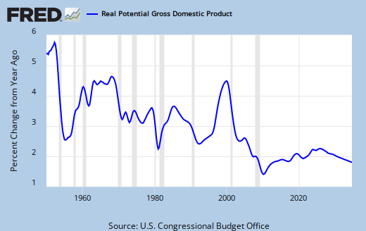
The first year on Graph #5 below shows the compound annual growth rate for the period 1947-1967. The second year shows 1948-1968. The last year shows the period 1991-2011. Each data point plotted considers the 21-year period is is centered in. Each point is a measure of two decades of Real GDP growth.

Graph #5: A 21-Year Moving Compound Annual Growth Rate
The growth rate starts high, above 4 percent. It ends low, barely above 2.5%.

The linear trend line shows a decline from over 4% growth to less than 2.5%. The red data line follows the path of the black trend line consistently from 1957 to 2001. There has been a gradual, long-term decline of economic growth.

Remember, this is a 21-year moving compound annual growth rate, and any given point is a measure of the growth that occurred from ten years before to ten years after that point. The low in 1983, for example, measures U.S. economic growth from 1973 to 1993. The high point in 1959 measures growth from 1949 to 1969.

There can be no question that economic performance was better early than late. There can be no question that the trend of real economic growth was consistent decline.


Early growth is consistently better than later growth. The overall trend of growth is down. There has been a gradual, long-term decline. There is no doubt that economic performance was better early than late.

And to Marcus I must say: I cannot accept your casual assertion that only the decade of the 1960s had anything like "golden" growth. Nor can I accept your Friedmanesque assertion that what looks like good growth was really no more than the precursor to inflation. I will continue to look upon the golden age as beginning even before the 1950s, after the second World War, around 1947.

And I will continue to assert that there was a weakening of economic performance as early as 1966-67 and this, rather than 1973-74, defines the end of the golden years.

By the way, I just discovered that Minsky said the same thing about the end of the golden age. Steve Keen writes:

We commenced deleveraging from 303% of GDP. After 3 years it is still 10% higher than the peak reached during the Great Depression. On current trends it will take till 2027 to bring the level back to that which applied in the early 1970s, when America had already exited what Minsky described as the “robust financial society” that underpinned the Golden Age that ended in 1966.

I love it when that happens.

// The Excel file with the StepRate function in VBA.

Monday, July 23, 2012

Economic Performance: The Record


I found this old post (dated 7 March 2011) on my 'development' blog, where I put ideas together and check my spelling and stuff. Apparently I never posted this one. I'm ready now.

By the way: I do not accept for one second the old Time magazine claim that the "skillful" economics of the time had anything to do with the economy's performance. However, I do accept that the economy's performance was very good at the time.

In addition, let me emphasize the view implicit in Paper Money, that stagflation has nothing to do with raging inflation. Stagflation is the occurrence of inflation even during recession -- a "hybrid" outcome, Smith calls it.

For source information on some of the excerpts, hover over the text.


Magnificent Success
"You have to have lived in the 1950s and 1960s to have
experienced a good economy." -- Jude Wanniski, 1995

My economics, my explanation of the economic problem, paints a picture. It shows a history of the U.S. economy that goes back to when times were good.

In the Robert Lucas post, I quoted Wikipedia: Lucas "challenged the foundations of macroeconomic theory (previously dominated by the Keynesian economics...)." That's part of the picture.

The six decades since World War II flake out as three decades of Keynesian economics followed by three of Reaganomics or (as I call it now) Wanniski-nomics. The three of the Keynesian era include two good ones -- the '1950s and '60s -- and the not-so-good '70s.

The festering of the not-so-good gave us Robert Lucas and Jude Wanniski and Ronald Reagan and Reaganomics. Wanniski-nomics. Things got better for a while then. But of course there was the debt. And now, after thirty years of Wanniski-nomics, things are not so good anymore.

And of course, there is the debt.

Magnificent Success
Highlights from an article in Time magazine, 31 December 1965:

In Washington the men who formulate the nation's economic policies have used Keynesian principles not only to avoid the violent cycles of prewar days but to produce a phenomenal economic growth and to achieve remarkably stable prices. In 1965 they skillfully applied Keynes's ideas—together with a number of their own invention—to lift the nation through the fifth, and best, consecutive year of the most sizable, prolonged and widely distributed prosperity in history.

By growing 5% in real terms, the U.S. experienced a sharper expansion than any other major nation. Even the most optimistic forecasts for 1965 turned out to be too low. The gross national product leaped from $628 billion to $672 billion—$14 billion more than the President's economists had expected. Among the other new records: auto production rose 22% , steel production 6% , capital spending 16% , personal income 7% and corporate profits 21%. Figuring that the U.S. had somehow discovered the secret of steady, stable, noninflationary growth, the leaders of many countries on both sides of the Iron Curtain openly tried to emulate its success.

Says Budget Director Charles L. Schultze: "We can't prevent every little wiggle in the economic cycle, but we now can prevent a major slide."

A slide, of course, is not what the U.S. Government's economic managers have been worrying about in 1965; they have been pursuing a strongly expansionist policy. They carried out the second stage of a two-stage income-tax cut, thus giving consumers $11.5 billion more to spend and corporations $3 billion more to invest. In addition, they put through a long-overdue reduction in excise taxes, slicing $1.5 billion this year and another $1.5 billion in the year beginning Jan. 1.

If the nation has economic problems, they are the problems of high employment, high growth and high hopes. As the U.S. enters what shapes up as the sixth straight year of expansion, its economic strategists confess rather cheerily that they have just about reached the outer limits of economic knowledge. They have proved that they can prod, goad and inspire a rich and free nation to climb to nearly full employment and unprecedented prosperity. The job of maintaining expansion without inflation will require not only their present skills but new ones as well. Perhaps the U.S. needs another, more modern Keynes to grapple with the growing pains, a specialist in keeping economies at a healthy high. But even if he comes along, he will have to build on what he learned from John Maynard Keynes.

Failure
Time's praise was a kiss of death. As America's Adam Smith wrote in Paper Money:

That was the high point. The dragons of inflation and unemployment began to snort in their caves, and 'stagflation,' an awkward beast, a hybrid of inflation and stagnation, roamed without serious natural enemies. Cynics said there were two sure signs that the Keynesian era was waning. One was that Time magazine put Keynes on its cover....

Disarray
In his 1987 book Alan Blinder, a member of the Council of Economic Advisers in the Clinton era, wrote:

Unfortunately, macroeconomics has been in utter disarray since the Keynesian consensus broke down in the 1970s.

Blinder's view was shared by Robert Heilbroner, who expanded on the thought:

Keynesianism was the economics of the world from around 1940 through the 1970s, but in the 1960s and 1970s came this extraordinary and quite unexpected inflation. And that took the bloom off the [Keynesian] rose. The Keynesian schema, which had tremendously wide acceptance, had no theory of inflation.... Since then, no new view that anyone can agree on has emerged, and there has been a vacuum in terms of a defining picture of what the hell economics is.... In the history of economic thought there has never been such a prolonged period of intellectual disagreement.

So this was my picture of the economy: Unprecedented success, until an indefatigable inflation arose; this inflation resulted in failure; and then disarray. Unprecedented growth in the 1950s and 60s -- the "golden age" -- followed by inflation and stagflation and slow growth in the 1970s, results that undermined Keynesian thought and policy. And then the patchwork called Reaganomics.

Right or wrong, this was my picture of economic performance since the second World War.

Disarray
And then one day, there was Krugman:

Did The Postwar System Fail?

I’ve been posting about the contrast between the popular perception on the right that America had slow growth until Reagan came along, and the reality that we did fine pre-Reagan, in fact better; see here, here, and here. And what I’m getting as a common response — including from liberals — is something along the lines of, “That’s all very well, but by 1980 the postwar system was clearly failing, so what would you have done instead of Reaganomics?”

Which all goes to show just how thoroughly almost everyone has been indoctrinated by the current orthodoxy.


He included a little graph to show that "The Ford-Carter years look no worse — in fact, somewhat better — than the Bush years, especially if you look from business cycle peak to business cycle peak."

Krugman's post is from last May. Ten months ago. This has been bothering me for a while now, notions like "America had slow growth until Reagan came along" and "we did fine pre-Reagan." And the argument that the 70s were no worse than the Bush II years. And the rejection of the view that "by 1980 the postwar system was clearly failing." I started to doubt my picture of economic performance.

I might argue that the economy was up in the 1950s and '60s, down in the '70s, up in the '80s and '90s, and down again in the 2000's. That would fit Krugman's graph into my picture. But all was up in the air.

Was my picture distorted? Was Krugman's? Was it true, as Krugman says people say, that growth since the '80s has been good? Was it true, as Krugman says, that the Bush years as bad as the 1970s?

The most basic question was: What about growth? What happened with growth? Was there a golden age, a bad decade, and a great moderation thereafter? What does the history of our economic performance look like?

It came to a head, finally, after I came upon Stuart Staniford's Growth Was So Faster in the Post War Years. Staniford shows a log graph of long-term "Real Per Capita GDP" and says, "it's hard to read changes in small growth rates on a log graph."

He continues:

If we instead go to the BEA data, and compute the CAGR (compound annual growth rate) over the thirty year period 1950-1980, it was 3.63%, while the 30 year period 1979-2009, it was 2.66% (2010 is not available yet). So the last thirty years are a whole percentage point lower growth. And that's despite the earlier period including the very rough years of the 1970s.

I liked that, because it fits my picture: excellent growth in the 1950s and '60s, "rough years" in the '70s, then some improvement. But I want a better breakdown. How does the improvement since the '80s compare with the '50s and '60s? And how do the Bush years compare with the '70s?

Staniford then graphs "the ten year CAGR for the decade prior to each year," which shows the early decades significantly better than the later ones. But I have trouble matching up the years with the performance values on this graph.

The best fragment in Staniford's post was "CAGR (compound annual growth rate)." In a follow-up comment, he provided the calculation for CAGR. And, given the name of it, I could Google for more. Found some useful stuff.

Disarray
I need to know. It can't be ambiguous.

I need my picture of history to be true, for I can explain it. I can explain the growth of the 1950s and '60s, the stagflation of the 1970s, the improvement of the 1980s and '90s, the decline and crisis.

I need this history to be true, or I need to know that it isn't.