... and yet, there is some relation between GDP and unemployment

(Following up on the previous post)

From The Myth of ‘Jobless Recoveries’:

It is rare to call an economic relationship a “law.” But Okun’s Law has earned its name. In 1962, Arthur Okun found a relationship that has become enshrined in textbooks as Okun’s Law. The textbook version states when U.S. output dips one percent below its potential, unemployment rises above its natural rate by about half a percentage point.

Richard H. Serlin: "For people who care about unemployment, we’re still deep in recession."

In comments on the old Stephen Williamson post I looked at yesterday, economist Richard H. Serlin wrote:

Part of the problem is that we don’t care about just GDP, at all. We also care about unemployment. By the GDP definition we aren’t even in a recession, let alone the Great Recession. For people who care about unemployment, we’re still deep in recession. We need a definition for recession/depression that actually takes into account, you know, UNEMPLOYMENT! To see if the early 80s recession was worse, for most people the crucial comparison is unemployment, and how long, not GDP growth.

In fact with our current definition of recession/depression, unemployment could be 30% and if we have two quarters of GDP growth from the 70% who do have jobs, economists would say the Depressions over!

I don't usually look at it that way, but Serlin makes a great point.

Name-dropping (Hodrick, Prescott, Williamson, Ball, the CBO, and Bullard)

The other day I googled graph of hodrick-prescott trend for GDP. First thing that turned up was Stephen Williamson (of the St. Louis Fed)'s HP Filters and Potential Output. Unusual for a Williamson post, I could follow most of it.

Let me provide some background here, from A Summary of Alternative Methods for Estimating Potential GDP (PDF). First, under CBO’s Method for Estimating Potential Output:

CBO’s estimate of potential output is based on the frame-work of a textbook model of long-term economic growth, the Solow growth model.

Next, under Other Methods for Estimating Potential Output:

Statistical filters (such as centered moving averages, bandpass filters, the Hodrick-Prescott filter, and the Kalman filter) are often used to extract the trend from GDP directly.

Finally, under Advantages and Disadvantages of the Different Methods:

The statistical approaches also have their drawbacks. For the filtering methods, three shortcomings are significant. First, many of the filters do not benchmark their trends to any external measure of capacity. Therefore, unlike CBO’s results, their results can be interpreted as trend GDP but not as potential GDP. In other words, they do not yield an estimate of the level of output that is consistent with stable inflation.

(Emphasis in the original.)

The difference is significant. Potential output is supposed to show what GDP would be if the economy was running at the level where something (demand, maybe) isn't causing inflation, but it would be causing inflation if anybody put in just an ounce more effort. Or, as CBO has it, potential output is

an estimate of “full-employment” gross domestic product, or the level of GDP attainable when the economy is operating at a high rate of resource use.

Although potential output measures the productive capacity of the economy, it is not a technical ceiling on output that cannot be exceeded. Rather, it is a measure of sustainable output, in which the intensity of resource use is neither adding to nor subtracting from inflationary pressure.

A year back I was having trouble with The Myth of ‘Jobless Recoveries’, a guest post by Laurence Ball, Daniel Leigh, and Prakash Loungani, at Econbrowser.

Eventually I worked it out. The trouble turned out to be that the Econbrowser post was my first experience with "the statistical approaches" that "do not benchmark their trends to any external measure of capacity." After that, I started doing some Hodrick-Prescott calculations and understood that post a little better.

Anyway, Stephen Williamson writes

In studying the cyclical behavior of economic time series, one has to take a stand on how to separate the cyclical component of the time series from the trend component. One approach is to simply fit a linear trend to the time series (typically in natural logs for prices and quantities). The problem with this is that there are typically medium-run changes in growth trends (e.g. real GDP grew at a relatively high rate in the 1960s, and at a relatively low rate from 2000-2012). If we are interested in variation in the time series only at business cycle frequencies, we should want to take out some of that medium-run variation. This requires that we somehow allow the growth trend to change over time. That's essentially what the HP filter does.

Williamson then quotes Paul Krugman:

When applied to business cycles, the HP filter finds a smoothed measure of real GDP, which is then taken to represent the economy’s underlying potential...

But Williamson says Krugman has it wrong. Williamson says the same thing the CBO says -- Hodrick-Prescott shows the trend of actual GDP, not the trend of potential GDP:

The HP trend is no more a measure of potential than is a linear trend fit to the data. The HP trend was arrived at through a purely statistical procedure... How then could the HP trend be a measure of potential GDP? To measure potential GDP requires a model.

Stephen Williamson then turns about-face. He says, let's use the Kydland-Prescott model (which introduced the HP calculation to economists) to figure potential output:

If the model is Kydland and Prescott's, there is a clear answer to what potential is - it's actual GDP (and certainly not the HP trend). That model doesn't have a government in it, and was not intended for thinking about policy. What Kydland and Prescott's work does for us, though, is to allow us to consider the possibility that, for some or all business cycle events, there may be nothing we can or should do about them.

Think of actual GDP as the trend of potential GDP, Williamson says, and consider the possibility that there may be nothing we can do about our declining economy. Reminds me of something written by a guy calling himself Adam Smith in The Roaring '80s:

...the Keynesian revolution gave some hope that nations could do something about the 'economic blizzards' that had previously been considered as random as the weather.

Williamson is one of those who see the economic blizzards as like weather we can do nothing about. Can and should do nothing about. Why is this guy at the Fed?

Why is he even an economist?


Williamson's third graph:

Williamson's Third: The Log of Real GDP and the HP Trend Since 2000

He says of this graph:

In its attempt to fit the actual time series, the HP filter has done away with part of what we might want to think of as the recession, and real GDP in the first quarter of 2012 was more than 1% above trend.

By 2012, actual GDP is above trend. The output gap is gone, because the Hodrick-Prescott calculation pushed the trend line down in response to the Great Recession.

It is a fluke in the calculation. It doesn't mean everything is back to normal. It doesn't mean unemployment is back to normal. It doesn't mean the economy is booming again. It is a fluke in the calculation.

But you know what I think? I think that's where James Bullard got his "wealth shock" view. From a fluke in the calculation.


// Update 16 September 2014: My conclusion (Bullard got his 'wealth shock' view from a fluke in the H-P calculation) is confirmed in the July 2012 article Blog review: HP Filters and business cycles by Jérémie Cohen-Setton and Yury Yatsynovich:

"James Bullard pointed to these [Hodrick-Prescott] estimates – together with the fact that we don’t see deflationary pressures (see our review here) – as evidence that advanced economies are operating near potential, if not above."

"Tim Duy points that St. Louis Federal Reserve President James Bullard ... likes to rely on this technique to support his claim that the US economy is operating near potential."

But there is an "end point problem" with the HP calculation:

" Luís Morais Sarmento – economist at Banco de Portugal – explains that the end point problem results from the fact that the series smoothed by the HP-filter tend to be close to the observed data at the beginning and at the end of the estimation period."

And this:

"Tim Duy points that if you don’t deal with the endpoint problem, you get that actual output is above the HP trend..."

Yeah. I noticed this "end point problem" too. See How to Change the Past.

Technology, Productivity, Growth, and Cost

Technological advance drives productivity if cost permits, but cannot move productivity if cost prevents it. Cost also allows or disallows the growth of output. So it looks like there is a relation between productivity and output. In truth, the connection is not direct, but runs through cost.

Productivity, Growth, and Cost

In the year 2000 Alan Greenspan looked to improved productivity as the reason the economy was so good:

In the last few years it has become increasingly clear that this business cycle differs in a very profound way from the many other cycles that have characterized post-World War II America. Not only has the expansion achieved record length, but it has done so with economic growth far stronger than expected. Most remarkably, inflation has remained largely subdued in the face of labor markets tighter than any we have experienced in a generation.

A key factor behind this extremely favorable performance has been the resurgence in productivity growth.

Stands to reason. If we produce more per hour than we used to, and nothing else changes, then output will go up.

Yet only a couple years later, Greenspan was puzzled. Productivity growth was impressively good, but economic growth was not:

The increase in nonfarm business output per hour over the past year will almost surely be reported as one of the largest advances, if not the largest, posted over the past thirty years. We at the Federal Reserve, along with our colleagues in government and the private sector, are struggling to account for so strong a surge. We would not be particularly puzzled if the increases in output per hour were occurring during a period of very rapid economic growth, such as has often attended recoveries from steep recessions... But during the past year we averaged only modest economic growth.

Evidently, productivity growth is not the whole story when it comes to economic growth.

//

In the latter speech, Greenspan said

From an average annual rate of 1-3/4 percent in the late nineteenth and early twentieth century, it jumped to a 3-3/4 percent rate in the decade following World War I. Subsequently, productivity growth returned to a 1-3/4 percent pace. Then, for the quarter century following World War II, productivity growth rose to an average rate of 2-3/4 percent before subsiding to a pace of 1-1/2 percent annually from the mid-1970s to the mid-1990s.

And then, looking back over the latter 1990s from his 2002 perspective:

Over the past seven years, output per hour has been growing at an annual rate of more than 2-1/2 percent, on average, compared with a rate of roughly 1-1/2 percent during the preceding two decades.

It seems that good productivity and a good economy go together. Productivity was good in the Roaring '20s, and in the Golden Age following World War Two, and again in the boom years of the latter 1990s. Sure: Productivity drives economic growth. But that isn't the whole story. Economic growth also drives productivity.

Apparently, the state of the economy affects our ability to use technological advance to improve productivity. The Great Depression, for example, was a time when improved technology failed to feed into productivity and growth; in a footnote, Greenspan says:

In contrast to the boom in productivity after World War I, which many economists associate with a few key innovations, analysts usually ascribe the post-World War II boom to innovations in many sectors reflecting the diffusion through the private economy of (a) new technologies that appeared in the 1930s but were not fully implemented during the Depression, and (b) a gradual application to civilian activities of military-related innovations.

"New technologies that appeared in the 1930s but were not fully implemented during the Depression". So it seems that two things are true:

1. Improved productivity leads to an improved economy; and
2. A declining economy leads to declining productivity.

How can this be? If productivity is pushing the economy upward, how can the economy be pushing productivity down? Obviously there is more to the story. If productivity pushing the economy upward meets resistance, it is likely that something else is pushing the economy down, offsetting or undermining the effects of improved productivity.

Greenspan says lower costs are associated with improved productivity: "On a consolidated basis for the corporate sector as a whole, lowered costs are generally associated with increased output per hour."

I say that higher costs are associated with declining productivity.

Excessive financial cost pushes our economy down. It pushes productivity down.

Jimmy Carter on the Colbert Report: the Bible says you don't charge interest to a poor person

You probably knew that.

At this site I found a couple good quotes. This (Deuteronomy 23:19-20 ESV):

“You shall not charge interest on loans to your brother, interest on money, interest on food, interest on anything that is lent for interest. You may charge a foreigner interest, but you may not charge your brother interest...

That's pretty direct. And this one (Proverbs 28:8 ESV):

Whoever multiplies his wealth by interest and profit gathers it for him who is generous to the poor.

which sounds like moral justification for progressive taxation.

The relation between productivity and growth

From Why Have the Dynamics of Labor Productivity Changed? (PDF, 26 pages) by Willem Van Zandweghe, an economist at the Kansas City Fed:

In recent years, the U.S. economy has undergone a change in the behavior of productivity over the business cycle. Until the mid-1980s, productivity growth rose and fell with output growth. But since then the relationship between these two variables has weakened, and they have even moved in different directions.

Thought I'd take a look at that. Here are "percent change from year ago" patterns for inflation-adjusted GDP and Total Factor Productivity at constant prices:

Graph #1: Growth Rates of RGDP (blue) and TFP (not blue)

Wait a minute... RGDP is quarterly, TFP is annual. That makes the blue line more jiggy. It throws off the comparison. I can't make TFP quarterly, but I can show RGDP as annual values:

Graph #2: Annual-to-Annual, Growth Rates, RGDP (blue) and TFP

Wow. That's better. The similarity really stands out now. But I don't know about what Willem Van Zandweghe said. It's pretty easy to see productivity growth rising and falling with output growth. It's not so easy to see a change in that pattern since the mid-1980s.

Hey! I know what to do:

Subtract from Series A the average value of Series A, and then divide by the standard deviation for Series A, and then multiply by the standard deviation for Series B, and then add the average value of Series B.

I used OpenOffice Calc on data from 1951 thru 2011 to figure the average and standard deviation values:

Then I retrieved Graph #2 and plugged in the numbers. Not bad. I got a couple "mismatched parentheses" errors along the way, but FRED and I survived the ordeal. Here's the Christensen-fitted comparison graph:

Graph #3: The blue line (RGDP) Christensen-Fitted to the not-quite-red TFP line

The two lines are a close match. At a glance, they move up and down together. And I don't see any movement in different directions since the mid-1980s. So I don't know what Willem Van Zandweghe was talking about.

Okay -- next, I subtracted the Total Factor Productivity number from the fitted RGDP. Just by inspection, I don't see any obvious errors in it; I think the new FRED is coming around. As for the graph itself:

Graph #4: Christensen-Fitted RGDP less TFP

Looks like RGDP growth is declining relative to total factor productivity. Maybe that's the "different directions" thing Van Zandweghe wrote about.

What the last graph shows is that even when productivity is good, GDP growth is not as good as it used to be: Even when productivity is good, GDP growth is not as good as it used to be.


Related Posts

August 11, 2013	"the theoretical case behind NGDPT is quite weak"
August 12, 2013	dividing these series, each by its own standard deviation, will similarize the up-and-downs of the different series
August 13, 2013	He sees the size and the location of the up-and-down pattern as separate from the pattern itself.
August 14, 2013	The first step of Christensen's calculation...
August 31, 2013	some nifty stuff with averages and standard deviations, to "fit" one line to another on a graph
September 1, 2013	Christensen's Market Indicator has already been used as proof and disproof, and I'm still just checking the arithmetic.
September 2, 2013	Lars's numbers are ridiculously large and obviously in error.
March 18, 2014	FRED must use a calculation very much like this to scale and shift the right-axis numbers, when two axes are used on a graph.

The Boom of the 1990s

NBER presents U.S. Monetary Policy During the 1990s, Matt Nesvisky's review of Greg Mankiw's review of, well, of U.S. monetary policy in the 1990s.

Mankiw notes the low volatility of inflation, growth, and joblessness. Then too, "large supply shocks were uncommon in the 1990s" , and "Good shocks in fact were more common than bad." All told, Mankiw sees in the 1990s a combination of good policy and good luck.

Here's the piece of Nesvisky's article that that gets my full attention:

Also fortuitous was the behavior of the stock market, for not only were returns high but volatility was low, making the 1990s essentially the best time ever to be investing in Wall Street. Little evidence suggests the booming market played a large, independent role in monetary policy. Yet significantly, the bull market of the period preceded the acceleration of the productivity rate by several years, and the market can be a driving force of the business cycle.

"The bull market preceded the acceleration of the productivity rate by several years."

I went right away to FRED -- it seems to be okay when calculations of series data are not involved -- for a look at Dow Jones and S&P rate-of-change rates:

Graph #1: Stock Market Index Growth Rates

The thin vertical line between 1990 and 2000 is not a recession, but a date selector related to the date and market index values just at the start of the large increase which, to me, looks like the start of the bull market of the 1990s. That large increase occurs in 1995.

But that's not "several years" before the acceleration of the productivity rate! What was Mankiw thinking???

Dean Baker and John Schmitt describe a "nine-year 1996-2004 boom" in productivity. Bill C at Twenty-Cent Paradigms presents his own estimate and that of the Economic Report of the President; both show the boom beginning in 1996. In a 2002 paper, Robert J. Gordon refers to "The 1995-2000 productivity growth revival". These sources all place the start of the productivity boom in 1995 or '96 -- the same year or the year immediately following the 1995 date I have identified as the start of the 1990s bull market. In contrast to Mankiw's "several years".

Perhaps I have the bull market date wrong? No. The San Fransisco Fed's Dr. Econ (February 2001) offers this graph showing the bullish increase beginning in the fifth year after 1990 -- that is, in 1995:

Graph #2: The bull market of the 1990s (red) begins in1995

According to Matt Nesvisky, Greg Mankiw places the start of the bull market several years before the start of the productivity boom. According to me, Greg Mankiw is not correct.

But if you're looking for something that "preceded the acceleration of the productivity rate by several years" I've got a contender for you. It's my latest version of the debt-per-dollar ratio -- base-to-debt this time. I first presented it on 23 March in relation to potential GDP. I offer it again now in contrast the the bull market story of Greg Mankiw.

Graph #3: Base Money Relative to Total Debt (red) and Stock Market Measures

This graph is similar to Graph #1. I had to recreate it once due to my own lack of foresight, and a second time because FRED destroyed the graph after I tried to save it as a PDF. But I have the same three market series as before, percent change from year ago, left axis. And I've added the bolder red line, AMBSL base money divided by TCMDO debt, with the "percent change from year ago" transformation.

On Graph #3 you can see a tall, wide increase in base relative to total debt. It begins around 1990 and lasts into the mid-1990s. This burst of money growth (in a time of reduced debt growth) does in fact occur "several years" before the start of the stock market and productivity booms of the 1990s. In fact, the lines cross in the mid-1990s: the red base-to-debt line falling just as the market indices get a good uptrend going.

Here's the link. But FRED can't get the dates right.

Zoho: Debt, Growth, and Inflation

Dunno what I searched for, but it led me to an old (2012) Joe Weisenthal post with a really good name -- There's Only One Way To Fix The Deficit — And Actually It's Totally Painless. After some painful preliminaries, Weisenthal says

the primary driver of deficits is a lack of growth.

I agree.

Weisenthal's post is too long and shows too many graphs, as if he thinks his staying-power is enough to convince the reader. Ha. But he does get around to saying this:

Sadly, achieving growth is not trivial. So although it's the only meaningful solution to the deficit, there isn't agreement on the magic answer to get there.

The magic answer, of course, is to reduce private sector debt. But Weisenthal insists on writing about the Federal debt.


The same search led me to an old (again, 2012) Fictional Reserve Barking post, Evsey Domar's "On Deficits and Debt": A survival guide for making sense of today's economic challenges. Circuit writes:

Specifically, in his paper, Domar demonstrated that, in the long run, the ratio of debt to GDP will gradually approach the ratio of the fraction of GDP borrowed each year to the rate of growth of GDP. So, for instance, the US federal government borrowed approximately 7 percent of GDP in 2012. If the borrowing continued at the same rate and the GDP (in money terms) grows at 2 percent per year, the ratio of debt to GDP will approach 3.5; with a 3 percent growth, it will be 2.3.

Thus, Domar showed that "less attention should be devoted to the problem of the debt and more to finding ways of achieving a growing national income" (1945:415)

I totally agree with the focus on growing national income. And it ties in nicely with Weisenthal's focus on growth. But it's Circuit's first paragraph that gets my attention: the long run, the ratio of debt to GDP, borrowing 7% of GDP annually, and 2% GDP growth. These are things I can do in a spreadsheet.

I can test to see whether the ratio of debt to GDP approaches 3.5 with 7% deficits and 2% growth, and approaches 2.3 with growth at 3% like Circuit says. Running a test like that is not a mathematical "proof" but it helps make the results real for me, and that's worth a lot.

In the Zoho spreadsheet below, you can enter numbers in the yellow cells and watch the graph change after the thing recalculates. If you mess up the sheet, you can fix it by refreshing the page.

The default settings match Circuit's example. The 7 in yellow cell A2 represents Federal deficits each year equal to 7 percent of GDP. And the 2 in yellow cell A3 represents GDP growth of 2 percent per year.

Circuit says "in money terms". Not sure what he means by that. I think he means "nominal" but based on Circuit's presentation, I think Domar must have been talking about "real" (not inflating) growth. Inflation would change the value of the long-run ratio. As Weisenthal says:

nominal growth is all you need to reduce our debt burdens.

If real growth is 2% and inflation is another 2%, nominal GDP growth is 4%. Existing debt shrinks faster relative to GDP if GDP is inflating.

So I added a third yellow cell, cell A4, to hold the rate of inflation. The default value is zero, no inflation; therefore the red line that represents eroded debt is hidden by the blue line which does not consider inflation. Click cell A4, type the number 2 (for 2% inflation) and press the ENTER key to see the erosion of debt that Weisenthal is talking about.

Try higher GDP growth rates also, to see how better growth reduces the debt/GDP ratio. If it looks like the blue line didn't move much, it may be because the numbers changed on the vertical axis.

Give the graph a moment to refresh after you make a change.



Check me on the "Eroded Debt" calculation.

AMBSL/TCMDO and GDPPOT

Graph #1: Growth Rates, Potential GDP (red) and Base Money as a Percent of Total Debt

The blue line is generally well below zero for most of the years shown. That is, the growth of base money was consistently slower than the growth of total (public and private) debt.

The red line generally trends downward. In other words, the potential in potential output diminishes over time.

The one remarkable, large and sustained, actual increase in base-relative-to-debt occurs on the blue line between 1989 and 1996. In the midst of that increase, potential output turns and trends upward for a decade. This is a significant change in the pattern of decline shown by potential output.

The only other significant change in the decline of potential output is the uptrend that occurs between 1955 and 1967. Remarkably, this trend corresponds even more clearly to an uptrend in the base-to debt ratio.

Conditions were different in the 1990s and the 1950s. The changes in the blue line look different on the graph. But both periods show uptrend in the base/debt ratio. And both show uptrend in potential output.

If you think we need better growth, look at money and total debt.

It works about as well as everything else the Fed does

I think the new FRED goes astray as soon as you get an error while entering the formula. Unfortunately, if you want to type a-b you have to type the "-b" really fast. Otherwise, in the fraction of a second between typing the "-" and the "b" FRED will give you an error. That's not something new; the old FRED was a pain in the ass that way, too. But with the new FRED, after you get the error message everything falls apart.

I managed to "add data series" for total debt, and the federal portion, and the state-and-local government portion, all without error. The graph all the while showed the first series correctly.

Then by typing "-b" really fast, taking time to position my fingers, and typing "-c" really fast, I got the formula to be "a-b-c" without getting an error message. And the graph actually showed something that matched the formula.

I was trying to duplicate the U.S. debt portion of Steve Keen's "Change in Private Debt" graph that I showed yesterday -- change in private debt as a percent of GDP. So next I added GDP as series d. (FRED identifies the series by letter; the first one you select is "a", the next is "b" and like that.)

But now I had to change the formula to read "(a-b-c)/d". Here's where I made my big mistake. I used the backspace to delete the formula, and before I could type the "(" FRED gave me an error message. It was all downhill from there.

I ignored the error message and entered the correct formula. Amazingly, the graph looked okay. But Keen's graph shows change in debt relative to GDP. So I went back to the a, b, and c data (my three debt measures) and changed the units from "Billions of dollars" to "Change, Billions of Dollars". I just changed the three debt series, not the GDP series.

But when I looked back at the graph, it had figured "Change, Billions of dollars" for all four series, including GDP. The graph was all spikey and obviously not like Keen's graph.

From there, things only got worse. I removed the "-d" from the formula and clicked "apply". The graph changed correctly. Then I added "-d" to the formula and clicked "apply" again. But the graph didn't change. Even though the formula shows "(a-b-c)/d", the graph and the graph borders show only "(a-b-c)".

What else did I do? Oh yeah, I clicked "max" up at the top, above the graph, to set the date range. And FRED set the date range, all right. It set the start date equal to the end date. But the graph didn't change!

But, hey: That was on the 20th. Maybe it's all fixed by now.

Getting it

I saw one of those build-a-story things on the internet the other day. You know -- read what everyone else has written, and add a sentence to build the tale.

I think stories get told like that on serious blogs, too: economic and political blogs. It's like building a meem. (I'm spelling it "meem" from now on, by the way.)

You know, I don't like those stories. Not when it comes to politics and the economy. These things affect people's lives. We need something better than just good stories. We need the stories to be right.

//

You got this from me. I got it from Tom Hickey. Tom got it from Mark Buchanan.

"A picture makes it clear", Buchanan says: "the recession IS over". He presents

a graph showing that the level of private debt — an indicator of how much businesses and individuals are borrowing—is now going up again after a long decrease during the recent crisis.

It's a little funny... Buchanan thinks the level of private debt is "an indicator of how much businesses and individuals are borrowing". I think the level of private debt is a measure of how much we have borrowed in total (and not repaid). It's the changes in that level that show whether people are borrowing. It's like "present tense" versus "past tense".

Anyway, Buchanan got it from Steve Keen:

Figure 1: Deleveraging is over -- for the time being

Referring to that graph, Keen writes:

The period of private sector deleveraging that caused the crisis appears to be over. Debt is now not merely growing, but growing faster than GDP...

Looks right to me.

//

Keen's post is dated 10 March 2014. In a post dated 9 July 2013, Nick Rowe wrote

If you look at business cycles this way, as a trade cycle, in which the volume of trade rises in booms and falls in recessions, it is totally unsurprising that the volume of borrowing and lending should also rise in booms and fall in recessions...

What would be surprising and in need of explanation would be if trade in IOUs did not follow the same cyclical pattern as trade in other goods.

Neil Irwin tells me that trade in IOUs is increasing in the US. (HT Mark Thoma). He's right that it's good news.

Nick Rowe got it from Marc Thoma. Marc Thoma got it from Neil Irwin.

//

Okay. Let's put a date on the "taper". From the Financial Times Lexicon:

"Taper talk" started in June 2013 when speculation increased that the Fed would start on a tapered end to QE in 2014. The increase in bond yields had already inflicted heavy losses on bond investors.

So, June. A month before Rowe and Thoma and Irwin. I think I know where Irwin got it. Irwin got it from the Fed.

But where'd the Fed get it?

Hmmm...

They updated Potential GDP last month

Real Potential Gross Domestic Product (GDPPOT) is now given in 2009 dollars. Before the February 4, 2014 revision it was given in 2005 dollars.

A lot of other series, including Real Gross Domestic Product (GDPC1), changed to 2009 dollars back in July of last year. Potential GDP has finally caught up, so now Real GDP and Potential GDP are directly comparable at FRED again.

Graph #1: Real (blue) and Potential (red) GDP, in 2009 Dollars

Here's how the two series looked, using the older data expressed in 2005 dollars:

Graph #2: Real (blue) and Potential (red) GDP, in 2005 Dollars

Not a lot of difference. The output gap there after 2008 closes a little more with the newer data. But not as much as I expected in a previous post. Why?

The "comprehensive revision" that changed Real GDP after the 2013-06-26 release didn't only change the base year from 2005 to 2009. It also increased the output numbers. It made Real GDP bigger than it was before. (Nice trick, huh?) So then, Potential GDP also had to be revised upward, to match the change in Real GDP. I didn't account for this change in Potential GDP. So the output gap doesn't close as much as I said it would, in that earlier post.


In order to compare the two versions of the output gap, I subtracted Real GDP from Potential GDP using the 2005-dollar data, and again using the 2009-dollar data, and put the results together on a new graph. Over the full period, the two "difference" lines run quite close together, as you might expect. So I zoomed in on a detail -- just the years since 2007:

Graph #3: The Output Gap using Old (blue) and New (red) data

The main thing you can see on this graph is that since 2009, the output gap gets smaller faster for the new (red) data than for the older (blue) numbers. That is what you have to expect, given CBO policy that reduces any output gap to zero in ten years:

CBO: A Summary of Alternative Methods for Estimating Potential GDP (PDF)

The surprising thing you can see on the graph is that, since 2007 or before, the new numbers show a bigger output gap than the old numbers. Not a lot bigger, but bigger. That's surprising, because Jim Bullard's argument was that Potential Output was over-estimated in the 2000s. Bullard's argument was that potential output was lower than people thought, that GDP was above potential, and that the shocking fall in Real GDP was really just a correction.

Now, it seems, they get to have it both ways: The output gap was bigger than people thought, but it's closing faster anyway.

ƛ

Yesterday I took the growth rate of employment, scaled it to the same amplitude as the growth rate of household debt, and centered the one line on the other. This process stripped away differences between the two lines, other than differences of pattern. That permitted me to compare the patterns of the two datasets.

So then I subtracted the one from the other, to see the difference. The blue line on the graph below shows the difference value. The red line is a Hodrick-Prescott trend line:

Graph #1: "Fitted" Employment Growth Date Less Debt Growth Rate (blue)
and a Hodrick-Prescott Trend (red)

You might have expected to see something like this:

Graph #2: The same data, but the HP calc uses a different value for  lambda

Almost the same. The blue line is the same. The red line is a little bit more wiggly. The big difference is in the legend, where the lambda value has changed from ten thousand to sixteen hundred.

The lambda is a constant used in the HP calculation. I don't know why they call it lambda. But it seems to be pretty important. It seems to be always reported in the notes that accompany graphs that show HP trend lines.

As I noted almost a year ago now, there is apparently a "rule of thumb" for picking a lambda value. It depends on the frequency of the data. For yearly values, a low number (100), for quarterly data higher (1600), for monthly data higher yet (14400).

I already know, from looking at the two graphs above, that the lambda value determines how much "smoothing" you get in the graph. A higher number gives more smoothing.

So I thought I'd look at a variety of lambda values, all applied to the same data. The source data here is quarterly, which means the rule-of-thumb lambda constant would be 1600. Here's what happened when I changed the constant:

Graph #3: Lambda = 100

Graph #4: Lambda = 1000

Graph #5: Lambda = 10,000

Graph #6: Lambda = 100,000

I used to think I should stick to the rule-of-thumb values as a rule. Now I think those values are just a starting point. If I really want to see the trend, I can increase the lambda until the little wiggles go away. And yeah, if you're going to be using non-standard lambda values, then that's a good reason to always report it in the notes that accompany the graph.

//

Preview or Download the Excel file from Google Drive. Note that the file contains my Visual Basic macros for formatting my graphs, and Kurt Annen's Visual Basic for the Hodrick Prescott calculation. Also, above the graph it says 1600 LAMBDA. Change that number from 1600 to some other value, and you change the graph.

// Update 30 March 2014: For my intro to the Hodrick-Prescott calculation, a link to an Excel add-in, a how-to-use link, and a link to some tips, see De-Trending.

I can picture what I want to do. Now I have to find the words...

Here's the second graph from 4AM yesterday, Troy's graph tweaked:

Graph #1: Percent Change from Year Ago, Employment (blue) and Consumer Debt (red)

I said it shows "two lines that run pretty close together except in the 1960s and the 1990s". So I started thinking about subtracting the one line from the other, to look at where the differences arise. You never know if something like that will turn out to be interesting.

That's what makes it so interesting.

Yeah, two lines close together. Except they're on two different axles. Two different axes. The lines are pretty close together, but the numbers themselves are not. Where the blue line is zero, the red line is seven. Where the blue line is 10, the red line would be 23. The numbers are not usefully close. But the patterns are teasingly similar -- and yet intriguingly different during the 1960s and 1990s, the two decades of above-average economic performance. Intriguing.

Then I remembered a technique I learned from Lars Christensen. It goes something like this:

Subtract from Series A the average value of Series A, and then divide by the standard deviation for Series A, and then multiply by the standard deviation for Series B, and then add the average value of Series B. At that point no further adjustment should be needed for comparing A and B.

That set of calculations I call "Christensen-fitting" the data. I don't know if it's a standard technique (and if so, what the name of that technique is) or if Lars Christensen invented it. But I like it.

So I downloaded the data from FRED and set to work.

I went right back to FRED then, changed the monthly PAYEMS series to quarterly so it matched the debt series, and downloaded the data again.

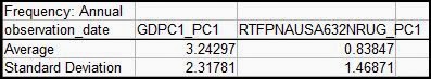
The CMDEBT data was intermittent before 1952Q4, so I deleted the data for both series before that date. Then all I had to do was find a spreadsheet with the calcs Christensen used, and duplicate the calcs. He used the STDEVPA() and AVERAGE() functions, so I did the same. Here are the numbers I came up with:

Next, I went back to FRED and plugged in the numbers for the Christensen-fit. Here is the result:

Graph #2: The Christensen-Fitted Version of Graph #1

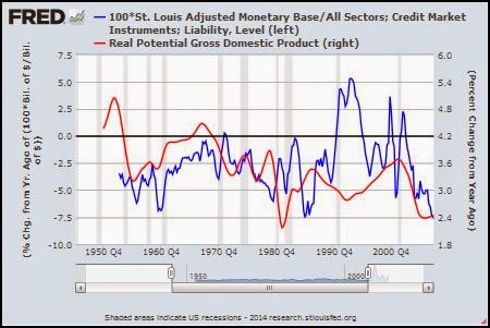
This graph looks very much like Graph #1 above. The difference is that now both datasets use the left axis. The PAYEMS numbers have been scaled and shifted to match the CMDEBT numbers.

(Hm. FRED must use a calculation very much like this to scale and shift the right-axis numbers, when two axes are used on a graph.)

Okay. Now that I have the employment numbers fitted to the debt numbers, I can subtract the one set from the other and see the difference:

Graph #3: "Fitted" Employment Growth Date Less Debt Growth Rate

Now it's getting interesting. Uptrend to about 1966. Downtrend to about 1980. Uptrend next, but not as rapid as before. Or maybe it's a low plateau in the 1980s and a higher plateau in the 1990s. And then a big drop -- but the big drop occurs about a decade before the crisis. Now that's interesting.

I subtracted the debt growth rate from the employment growth rate. So where the line is below zero, debt growth is the bigger number. Again, where the line is below zero, the debt growth rate was faster than the employment growth rate... Well, I have to be careful here. The debt growth rate is always faster than the employment growth rate. If I go back to the first graph and put everything on the left axis, it looks like this:

Graph #4: Not Fitted, and On the Same Axis, Debt Growth (red) Is Way Faster

The debt growth rate is always a lot faster than the employment growth rate, except there at the end, after the crisis.

Well, yeah. That's why I fitted the one series to the other. So we could compare them. But I have to be careful how I talk about it. So let me try again:

On Graph #3, I subtracted the debt growth rate from the "fitted" employment growth rate. So where the line is below zero, debt growth is the bigger number. That is, where the line is below zero, the debt growth rate was faster than the "fitted" employment growth rate.

Where Graph #3 is below zero, the debt growth rate is relatively faster than the employment growth rate. Where Graph #3 is above zero, the employment growth rate is relatively faster than the debt growth rate.

Where Graph #3 shows a trend of increase (before 1967), the trend favors employment. Where it shows a trend of decrease (1967-1980) the trend favors debt growth.


I downloaded the "fitted" data from FRED, put it into Excel, and added a Hodrick-Prescott trend line to it:

Graph #5: Same as Graph #3 (blue) with a Hodrick-Prescott Trend (red)

(I'm repeating this graph in tomorrow's post. If you have any comments on my "lambda" value, save them up for that post!)

The trend favors employment till about 1967, then debt till 1980, employment till the mid-1990s, then debt again since maybe 2003 ...

The trend favors employment till about 1967. That's interesting, I think. I have it in my notes that Scott Sumner identifies the years 1952-1964 as a big debt surge. But despite surging debt, employment grew more. Can that be right?

Graph #6

No, of course not. Debt always increases faster than the number of jobs.

But look at it this way: From 1952 to the mid-1960s, employment was winning in a race of go-karts. At the same time debt was losing in a race among dragsters. Then from the mid-1960s to 1980 employment was losing among go-karts and debt was winning among dragsters. That's what Graph #3 and Graph #5 show, the Sumner debt surge of 1952-1964 notwithstanding.

Now look at it this way: The employment growth of 1952-1966 was faster, compared to employment growth of the whole 1952-2013 period, than the debt growth of 1952-1966 compared to debt growth of the whole period.

Debt growth in the early years was only moderate, as debt growth goes, while employment growth in those same years was very good, for employment growth.

Yeah, that's it.

I ♥ Steve Keen

From Closing the door on the GFC by Steve Keen, at Business Spectator:

... central banks hope they can “fine tune” the economy using the interest rate alone, and with US unemployment levels now within cooee of the level at which Ben Bernanke said monetary policy could return to “normal”, the Federal Reserve may start to increase rates in late 2014.

This belief that getting the interest rate right is all that it takes to keep the economy out of recession is the product of economic models, not of economic experience.

...when you look at the data, there isn’t much of a relationship between the interest rate and recessions...

But in fact there is a much clearer relationship when you include one factor that these models ignore: the level of private debt...

...look not at interest rates alone, but interest payments as a percentage of GDP...

You
may
have
heard
similar
things
from
me
Oh yeah, one more thing:

I thought it was a typo.

The new FRED

The pink error message appears to be something left over from the old FRED. Only it's missing a number. It should read like this:

Each data series can only combine up to 10 individual series...

My Data Series 1 has TWO individual series, only one of which appears on the graph, contrary to the "a/b" calculation I entered in a field you can't see in the image.

I got the error when I created Data Series 2, with only one individual series.

I miss the old FRED already.

I tweaked Troy's graph...

Troy linked to this graph in a comment on Jazzbumpa's Equity Extraction and Personal Consumption Expenditures:

Graph #1: Blue is YOY Job Gains, Troy says, and Red is YOY Consumer Credit Growth

Troy wants us to see the part where the two lines are similar, since about 2002, when employment was pushed up and dragged down by changes in credit use. I see it. But what catches my eye is the time before 2002, when job growth was high and debt growth was low. The "macroeconomic miracle" years.

I tweaked Troy's graph to look at more years, and to look at percent change. I got two lines that run pretty close together except in the 1960s and the 1990s:

Graph #2: Percent Change from Year Ago, Employment (blue) and Consumer Debt (red)

In the 1990s, the blue runs well above the red for near a decade. In the 1960s, the same thing happens. Two particularly good decades, the sixties and the nineties. And Troy's graph shows it.

Good graph, Troy.

We owe it to ourselves

Again, Steve Keen:

I couldn’t con­vince sev­eral of the aca­d­e­mics in the audi­ence of the impor­tance of pri­vate debt: they kept com­ing back to “one person’s debt is another person’s asset, there­fore the level of debt doesn’t mat­ter”.

Yeah... and I just ran across this, again, from Paul Krugman of all people:

... So, a few more thoughts on debt and what it does and doesn’t signify.

Start with the numbers that Stockman loves to cite, showing the ratio of total debt, public and private, to GDP...

Stockman, and to be fair quite a few people, would have us see this as evidence that we have been on a vast spending spree...

OK, the sheer size of that number should tell you immediately that this can’t be right. Yes, we have run trade deficits and moved from being a net creditor to being a net debtor, but it’s not that big a deal (and we still earn more on our foreign assets than we pay on our foreign liabilities). So the surge in debt reflects a surge in money Americans owe to other Americans.

Krugman: "the surge in debt reflects a surge in money Americans owe to other Americans."

There it is again, what Steve Keen said: One person's debt is another person's asset. We owe it to ourselves.


Okay. I went back and finished reading Krugman's post. He says:

This is how you want to think about debt: it’s not a burden on the nation’s resources, because it’s mainly money we owe to ourselves, and it’s a problem not because we have to tighten our belt but because debt is currently leading to spending that’s less than we need to maintain full employment.

The last part of that is good -- so good that I can almost overlook the we owe it to ourselves part. But if it is true that "debt is currently leading to spending that’s less than we need to maintain full employment", the growth of debt is the reason.

Krugman acknowledges that debt has grown, but seems to miss the point that it was the growth of debt that gradually undermined the spending we need to maintain full employment. He gets the ending: There was a moment, all of a sudden, when unemployment shot up and an output gap opened. And he can see that the high level of debt was the cause of it.

But debt didn't suddenly jump to a high level and cause the sudden opening of an output gap. Debt was creeping up for a long time, having a harmful effect on growth for a long time, until a final straw broke the camel's back and created the output gap. Debt was excessive -- meaning "debt was hurting the economy" -- for a long time. A long time.

Graph #2: Stages of the slowdown in real growth

Krugman doesn't seem to see it. He says debt is "currently" causing problems. But there is so much more to the story.


Oh, and the other thing: "debt: it’s not a burden on the nation’s resources, because it’s mainly money we owe to ourselves". I don't know what the hell that means: "a burden on the nation's resources". Resources? Debt is a burden on the people who owe it. Even though we owe it to ourselves. Or, to each other. Or, the many of us owe it to the few of us. Whatever.

No matter who we owe it to, the money we pay for our debts is money that goes to finance rather than to labor or to productive ("nonfinancial") business. The money we pay for our debts adds to cost without adding to output. Oh, yeah, we may use that money to produce stuff, or to buy stuff; but we could as easily have used our income for those purposes instead of borrowed money... As easily, or more easily, if policy encouraged it. But policy does not.

Policy encourages saving. Why? I do not know -- Maybe so banks have money to lend?? But hasn't that logic been shot down? So, policy encourages saving for no reason. No economic reason. Policy encourages saving because people like the idea, maybe. It's not a policy that actually helps people save, but nobody seems to get that. Eh, regardless, policy encourages saving.

When money goes into saving, money goes out of circulation. Funny thing is, it's money in circulation that we receive in our paychecks. The money in circulation is money that becomes income. Savings can't be income, because savings is not in the spending stream. Only circulating money flows.

A policy that encourages saving is a policy that makes less money available for use as income. Such a policy has multiple effects. It helps to limit increases of income. So you could say it is a way to fight inflation. Or you could say it prevents incomes from keeping up with the cost of living. Probably both those things are true.

The encouragement of saving also helps credit use grow. Do banks lend out savings?? Regardless, encouragement of saving shifts money out of circulation, creating a shortage of money in circulation. That is a problem people solve by borrowing more. So the encouragement of saving encourages borrowing and encourages the growth of accumulated debt.

So here ya go: Policy encourages saving, which creates a shortage of circulating money, so we increase our borrowing and our debt. Again: less circulating money, and more debt.

Graph #3: Less Circulating Money and More Debt Push the Debt-per-Dollar Ratio Up

From five dollars of debt for every circulating dollar, to more than $15 by 1990, to more than $35 by the time of the crisis.

The cost of a loan depends on the interest rate you can get. But for the economy as a whole, the cost of finance depends on two things: interest rates, and the level of debt accumulation.

The level of debt matters, because it affects the macroeconomic cost of debt.

Type stuff in the yellow cells

I want to look at accumulated debt as a percent of GDP in 1955 and in 1980 and in 2005. I want to use ceteris paribus and assume the rate of interest is constant: We know interest rates are not constant in the real world, but we need to focus on something else at the moment -- we need to focus on the accumulation of debt -- and the effect of varying interest rates is something we can look at later.

Given a load of debt at say a 5% rate of interest, the cost of that debt varies with the level of debt relative to GDP.



According to one reliable source, debt was 132 percent of GDP in 1955, 159 percent of GDP in 1980, and 311 percent of GDP in 2005. Plug those numbers into cell D2 of the spreadsheet, and note the changes in the cost of debt as a percent of GDP.


Assuming a constant 5% interest rate, total interest cost in 1955 amounts to 6.6% of GDP; in 1980 to 7.95% of GDP; and in 2005 to 15.55% of GDP. We assume no change in the interest rate, so the increasing cost of debt shown here is due entirely to the increasing accumulation of debt.

Blowin' in the Wind

In a recent look at trends of total factor productivity at Twenty-Cent Paradigms, Bill C linked to two NBER papers by Robert Gordon. One paper, and an update.

NBER provides access to abstracts of those papers for free, so that's what I'm looking at. The first paper is Is U.S. Economic Growth Over? Faltering Innovation Confronts the Six Headwinds. The phrase "six headwinds" catches my eye; it promises a summary view of problems that, in Robert J. Gordon's view at least, interfere with economic growth:

Even if innovation were to continue into the future at the rate of the two decades before 2007, the U.S. faces six headwinds that are in the process of dragging long-term growth to half or less of the 1.9 percent annual rate experienced between 1860 and 2007. These include demography, education, inequality, globalization, energy/environment, and the overhang of consumer and government debt.

"And the overhang of consumer and government debt." Last, but not least.

But you know what? Robert Gordon expresses concern only with consumer debt and government debt. He doesn't express concern with the debt of farm business or nonfarm noncorporate business or nonfinancial corporate business. Nor does he express concern over the many components of domestic financial debt. Yes, concern with any debt (other than the tiresome focus on only government debt) is something to be thrilled about. But still...

Graph #1: Consumer and Government Debt as a Percent of Total Debt

The debt that concerns Robert Gordon is less than half of credit market debt, and until the crisis was a decreasing portion of it.

Yeah... So what does Mr. Gordon say in the update?

The primary cause of this growth slowdown is a set of four headwinds, all of them widely recognized and uncontroversial. Demographic shifts will reduce hours worked per capita, due not just to the retirement of the baby boom generation but also as a result of an exit from the labor force both of youth and prime-age adults. Educational attainment, a central driver of growth over the past century, stagnates at a plateau as the U.S. sinks lower in the world league tables of high school and college completion rates. Inequality continues to increase, resulting in real income growth for the bottom 99 percent of the income distribution that is fully half a point per year below the average growth of all incomes. A projected long-term increase in the ratio of debt to GDP at all levels of government will inevitably lead to more rapid growth in tax revenues and/or slower growth in transfer payments at some point within the next several decades.

He reduces six headwinds to four. And he abandons concern with private debt.

1. Demographic shifts: People are exiting from the labor force because the economy is so bad. Fix the economy, and you'll solve Robert Gordon's demographic problem.

2. Education: Again, fix the economy. Make it so that there's a chance getting an education will be beneficial. Make it so that you can get a damn job when you get out of school. This will fix Mr. Gordon's second headwind.

3. Inequality: The growth of inequality is a result of the supply-side policies imposed on our economy since the late 1970s. Those policies were put in place to solve a problem. The policies didn't solve the problem, and they created a new problem. Get rid of those policies, and you eliminate Mr. Gordon's third headwind of four.

4. Government debt: Government debt? No. Private debt, or maybe all debt. But certainly not just government debt.

Fix the economy. Create policies that discourage the accumulation of private debt. Tear down this wall of policies that encourage the accumulation of private debt. Reduce the cost of finance. That's all we need to do. And then eliminate the "fixes" we put in place, that created inequality and globalization and other problems.

The rest will take care of itself.

I can't let this go, Tom

In The Real Ponzi Scheme: Private Debt at Asymptosis (from 2011), we read:

Economists will tell you that gross debt levels don’t matter because one person’s debt is another’s holdings. (Net: zero.) They ignore it.

But if the gross private debt is too large, the real assets in the real economy can’t generate enough income to pay it off. Not really complicated, conceptually.

My reply:

“Economists will tell you…”
Second time I’ve heard that, lately. Got a link or two handy?

I was having a hard time believing that anyone would say gross debt levels don't matter. Steve Roth provided a link; Steve Keen speaking:

One part of the dis­cus­sion that I found quite notable was that, even after show­ing empir­i­cal evi­dence on the impact that ris­ing and then falling pri­vate debt had on the econ­omy both now and dur­ing the Great Depres­sion, I couldn’t con­vince sev­eral of the aca­d­e­mics in the audi­ence of the impor­tance of pri­vate debt: they kept com­ing back to “one person’s debt is another person’s asset, there­fore the level of debt doesn’t mat­ter”.

In the years since, I've come to see that too many people say gross debt levels don't matter because it all nets out to zero.

(Scratching my head) Where've I seen that recently?

Oh, I know. Tom at Mike Norman's:

These morons apparently don't realize that all money is created by crediting and debiting accounts. Money functions as a unit of account, medium of exchange, store of value, and record of debt. Every debt has a corresponding credit denominated the unit of account of that jurisdiction, so that all debt as someone's liability is someone else's asset, which nets to zero.

No, Tom. You're emphasizing the wrong things, and you are leaving out cost.