Sunday, October 12, 2014

Tedium


I want to look at each of the images used for yesterday's animation sequence. Each of the similarities, I mean. But I'm having a hell of a time getting started with the writing. So I'm gonna just start.

Image #1: No lag... Similarity: January 1919 - November 1930

Graph #1: No Lag
I'm using another FRED graph, monthly data, same two series shown in the animation sequence, to see the dates of similarity. Maybe that'll move the writing along.

I will describe a "lag" in terms of how many months I have to offset the Base Money (black) graph to the right to obtain a highlightable period of similarity. I will describe a "similarity" using the dates of the Inflation (red) graph, the one that doesn't move back and forth thru time.

The similarity highlighted in Graph #1 ends suddenly in late 1930, when it appears the Federal Reserve suddenly decided to do something about the Great Depression. Just after the yellow highlight ends, base money (black) shoots up while the rate of inflation falls for six months more (till June 1931) and then drags bottom at -10% till March 1933.

That separation of the lines shows the lag developing.

Image #2: Lag 29 months... Similarity March 1933 - March 1934

Graph #2: Base Money Lagged Two Years
During the similarity highlighted on Graph #2, base money (black) increased from November 1930 to October 1931 -- a period of eleven months. The rate of inflation (red) increased from March 1933 to March 1934 -- twelve months. So the lag itself was a month longer at the end of the similarity than it was at the start.

At the start of that similarity the lag (November 1930 to March 1933) was 28 months. By the end of that similarity, it was 29 months. I'll call it 29 months.


Image #3: Lag 50 months... Similarity March 1934 - May 1937

Graph #3: Base Money Lagged Four Years
On Graph #3 the similarity starts with the peaks that end Similarity #2. The lag this time is clearly visible as a downtrend that's twice as long for the red as for the black, followed, then, by a more hesitant red uptrend. The similarity ends with rather modest peaks in both the red and black lines.

Note -- This image has been revised. Originally I showed one yellow stripe of highlight, running through those modest peaks. (You can see that version in yesterday's post.)

Incidentally, the peaks that end Similarity #2 no longer appear aligned because on Graph #3, base money (black) is shifted two additional years to the right. (If that doesn't make sense, go fiddle with the interactive experiment graph again.)

The end of this similarity is the highlighted peak of the black line in March 1933. And for the red line, in May 1937. The difference -- the time the black line is lagged -- is 50 months.

Image #4: Lag 63 months... Similarity May 1937 - October 1938

Graph #4: Base Money Lagged Five Years
Number four is a brief similarity. I'm figuring that it runs from the end of Similarity #3 to the start of the highlighted jiggles just before the black line skyrockets.

For the black line it starts with the end of Sim #3 (March 1933) and ends in July 1933.

For the red line it starts with the end of Sim #3 (May 1937) and ends in October 1938.

It's a challenge to get the dates right on these graphs, what with these images lagged (but not providing pop-up info windows) and the FRED graph providing the info windows (with nothing lagged). It's making my head spin. Hey, if you see anything that looks like a mistake, let me know.


Image #5: Lag 92 months... Similarity October 1938 - March 1951

Graph #5: Base Money Lagged Seven Years
For this one the similarity will start with the jiggles where the previous similarity ended. So July 1933 for the black line, and October 1938 for the red, these dates mark the start.

Where to end this similarity? For the black line I'm gonna go with the high point in the third tall spike in the group of three, so July 1943

For the red line I'm gonna stop it at the top of the third red spike of three, March 1951.

The highlighting is a bit off from these dates that I'm choosing now. It's a little bit arbitrary, choosing the dates. If you know a better way to figure it, do let me know.

(It's completely arbitrary.)

Image #6: Lag 74 months... Similarity March 1951 - March 1955

Graph #6: Base Money Lagged Six Years
We reached a maximum lag of 92 months (between 7 and 8 years) with Graph #5. On graph #6 the lag begins to recede. I'm calling the dates for this similarity as follows: For the black line, start at November 1944 and end at September 1949.

For the red line, start at March 1951. And end at, I'll say March 1955

For the red line, I start Similarity #6 where #5 ended. For the black line I'm leaving a little gap. Number six starts at the black peak where the yellow highlight starts. But number five ended at the nearby, higher, slightly earlier peak. So there is a brief gap between similarities at that point.

Note that other than this brief gap, and the dis-similarity described under Image #1, there are no gaps where one similarity ends and the next one begins. Granted, this is all by eye, and arbitrary. But these "similarities" are nothing but short sections of the overall graph, short enough that we can compare them and describe them.

But if the similarities connect like railroad cars, then what we're seeing is that the pattern of the red graph and the pattern of the black graph are actually quite strikingly similar. The main difference between the two lines is nothing more than a lag -- a long and variable lag. And I'm thinking that the best way to show similarity would be with an "accordion axis" if I knew how to make such a thing.

I'm also thinking that this accordion axis would essentially be a standard axis modified by a calculation that shortens or lengthens the time units in an irregular pattern. I want to create such an axis, because I want to take that calculation and see what it looks like as a normal graph. If it has a familiar look, if it reminds us of something, then perhaps we will have found a major component of the rise and fall of this lag.

Image #7: Lag 60 months... Similarity March 1955 - May 1960

Graph #7: Base Money Lagged Five Years
On Graph #7 the lag recedes again. I begin Similarity #7 where similarity #6 ended: September 1949 for the black line and March 1955 for the red. I end the red one in May 1960. And I end the black one at May 1955. We end with a five-year lag.


I figured these start- and stop-points by looking for similarities in the patterns. Tomorrow I'll graph the lag lengths.

Saturday, October 11, 2014

The Ridges on the Rocks


Maybe you need an accordion axis. Or maybe the lag amounts mean something.

There is a story I like very much, told by Lionel Ruby in "How the Scientist Thinks":
Darwin and a fellow scientist were searching for fossils in the north of England. They were not aware of the glacial theory at the time. Years later Darwin revisited the area, and he was now astonished to discover how clearly marked were the glacial ridges on the rocks. He had not noticed them on his earlier visit because he was not looking for them.... Darwin was able to appreciate the glacial markings only after he became aware of the glacial theory.


Sure: If the glacial theory was wrong, knowing about it and looking for it would still have led some people to see it in the rocks. But that's the trade-off, isn't it. If the glacial theory is right, and you don't know about it, you may not see it even if it is clearly marked in the rocks. Even if you are Darwin.

Me? I'm just lookin at the economy.


From the interactive experiment I captured some images with different lag values. On each image I highlighted in yellow the the part where I think the two graphs match. Some are obvious. Some may be a stretch. It's all by eye anyway; this is conceptual economics. But hey, it can't be any worse than the stuff that passes for "mainstream".

Slide your mouse back and forth across the Animation Bar below the graph:

Lagged Effects of Base Money: an Animation

Zero Year  Lag Two Year  Lag Four Year  Lag Five Year  Lag Seven Year  Lag Six
Year  Lag 
Five Year  Lag 

Now I want to show you the ridges in the rocks. I want to show you what I see.

First, notice that the red line does not move when you drag the mouse across the Animation Bar. The red line is the same in every frame because inflation is a resultant and because the history of inflation is what it is. As your eyes pass over the red line from left to right, you are simulating the passage of time.

Second, notice that the yellow highlight moves from left to right as you drag your mouse from left to right across the Animation Bar. The yellow highlight directs your focus to "similarities" between the red and black plot lines on the graph. The similarities are highlighted left to right because I tend to read graphs from left to right, again simulating the passage of time.

To my mind, the similarities offer a way to measure lag: Slide the Base Money graph over the Inflation graph until you find similarity. Then observe the distance you moved the graph. On our horizontal axis, that distance is a measure of time. It is the time it takes for the pattern of the one graph to show up on the other. We are measuring lag.

Third, notice that the black plot line, the Base Money plot, moves as you drag your mouse from left to right across the Animation Bar. At each step, the black line is offset a number of years from chronological time; this offset is the lag.

Granted it's all done by eye, and the annual steps are large and ungainly. Still, we are only attempting to observe similarities between two data sets -- and this is no more than common practice. What's odd is that the similarities show themselves separated by "large and variable" lags.

In order to see the similarities we need to develop an "accordion axis". For if you observe the movement of the black line as you move the mouse across the Animation Bar, you will notice that the black line moves first from left to right and then from right to left. The "similarities" depend at the start on an increasing lag, and, by the end, on a decreasing lag.

I am arguing that an increasing lag is associated with a slowing economy and that a decreasing lag is associated with a recovering economy. I am preparing to argue that the size of the lag is proportional to the severity of the economic slowdown.

Friday, October 10, 2014

I'm gonna agree with Milton Friedman on this...


From JSTOR's Friedman on the Lag in Effect of Monetary Policy by J. M. Culbertson:


I'm thinkin', like when you make the water hotter, in the shower, and nothing happens, so you turn it up more, and all of a sudden it's too hot. But whether it gets too hot or not depends on other things, too: Did the water heater just finish a duty cycle, or is it almost ready to start?

I think we can relate the size of the lag to the pace of new credit use, or in particular, to the size of new credit use relative to the size of something -- GDP, or base money, or base plus Federal deficit spending, something. I don't need to resolve this immediately.

I do think we can predict can calculate approximately the relative lag between a change in base-money growth and a corresponding change in inflation. Look, I'm not making any promises. But this is what I want to explore.

Wouldn't it be nice to have a better idea how "lags" work?

Thursday, October 9, 2014

An Interactive Inflation Experiment


If you're worried (or not) about inflation resulting from the Quantitative Easing of Base Money since the crisis, you might want to be looking at the rate of inflation:

Graph #1: The Rate of Inflation since 1913
and at the rate of Base Money growth:

Graph #2: The Rate of Base Money Growth since 1918
The money numbers go back to 1918 -- the year my father was born, God rest his soul -- and the price numbers go back even farther, to 1913. The numbers for both are monthly (so there's a lot of data) but for today's graphs I'm using quarterly values and showing "percent change from year ago". Maybe that's more than you wanted to know. If not, you can click either of the above graphs to go to its FRED source page.

Graph #3: Rate of Inflation, 1918-1960, #MQp

Graph #4: Base Money Growth, 1918-1960, #MQo
I reduced the range of dates on both graphs so they start on 1 January 1918 and end on 1 July 1960. These dates center the Depression-era Quantitative Easing on Graph #4, and allow ten years or more before and after that QE, where cause or consequence might show up on the graph of inflation. Oh, and I erased the background and border of the Base Money graph to make it see-through. So now we can put the base-money graph on top of the Inflation graph and see the two plots together.

Plus, I figured out how to use buttons to move the one graph relative to the other.

You can use the buttons to look for patterns in inflation that match or don't match patterns in base money growth. The "zero year" button aligns the dates of the two graphs, 1930 atop 1930, 1940 atop 1940, and so on. The "1 year" button shows money growth lagged one year; the "2 year" button shows money growth lagged two years; and so on.

The "10 year" button aligns 1930 on the base money graph (black) with 1940 on the inflation (red) graph. You can check the x-axis dates to see what the buttons do.

Even before you click a button, notice that the two lines match pretty well in the early years (up to 1930). After that it's a jumble. So, click some buttons and look for pattern similarities, and have some fun with this thing.

bottom image
top image
Graph #5: Base Money Growth (black) Overlaid on the Inflation Rate (red)
Click a Button to Lag the Base Money Graph by the Number of Years Indicated.


NOTE: If the buttons don't work for you, try this post instead.

Here's what I see: When base money is lagged seven years, the three major increases in base money (1934-1946, black) align remarkably well with three inflationary peaks (1940-1953, red). With a seven year lag.

As I observed yesterday, it is now just six years since quantitative easing began, in September 2008.

During the Great Depression, it took seven years for the unusual pattern of base money growth to be echoed in the inflation pattern. It took seven years, in other words, for inflation to arise as a result of base money growth in the 1930s.

In this post I offer one conclusion: It is still too early to say no inflation will arise from the quantitative easing of our time.

Wednesday, October 8, 2014

Bragging Writes


The Writers versus the Signatories


At Bloomberg:
Signatories of a letter sent to then-Federal Reserve Chairman Ben S. Bernanke in 2010 warning of the risks associated with the bank’s policy of quantitative easing are standing by their claims -- even as the biggest U.S. companies are flourishing, inflation is muted and holding Treasuries has been one of the best trades out there.

In the word "even", you can read the position taken by the writers of that story:

Signatories stand by their prediction of inflation even as the economy improves.

The position taken by the writers is that the economy is doing better, and the improvement is evidence that inflation will not come, so the signatories were obviously wrong.

You see a lot of that lately: the idea that we have not had inflation yet, so we're not gonna get it. And yes, at some point you do have to say "The waiting period is over. A final outcome can now be determined." I'm just not sure we're there yet.

The writers continue:
The Nov. 15, 2010, letter signed by academics, economists and money managers warned that the Federal Reserve’s strategy of buying bonds and other securities to reduce interest rates risked “currency debasement and inflation” and could “distort financial markets.” They also said it wouldn’t achieve the Fed’s objective of promoting employment.

Four years later, members of the group, which includes Seth Klarman of Baupost Group LLC and billionaire Paul Singer of Elliott Management Corp., are facing a different economy. U.S. companies now boast low debt, big cash piles and record profits. They’re creating jobs at the fastest average pace since 2005 and unemployment has dropped to 6.1 percent from 9.8 percent when they wrote the letter. The recovery has underpinned an almost 200 percent gain in the Standard & Poor’s 500 Index since March 9, 2009.

Four years have passed, the writers point out. And, judging by that last paragraph, the economy is doing very well.

So, what do you think?

The economy is not doing well at all. Not the economy I know. But it is doing better than it was. And that is when the threat of inflation can become real -- when things pick up. The writers, laughing at the signatories and thinking we have not had inflation so we will not, those writers are on thin ice. That's what I think.

Inflation is held down by a depressed economy. If inflation picks up, it will happen when the economy picks up. Now, I'm not predicting inflation. But the view that says "the economy is doing better, so inflation is not a threat" is just exactly wrong. I can't see how people who write about the economy can pretend to believe it.


The question of timing remains. The writers point out that four years have passed since that letter was written, and the economy is doing fine. The implication is that if we were going to get inflation, we'd have got it by now.

What do you think? Is four years enough time? How about six years? It's four years since the letter, but it's a full six years since the start of Quantitative Easing. The quantitative easing that troubles the Signatories started in September 2008:

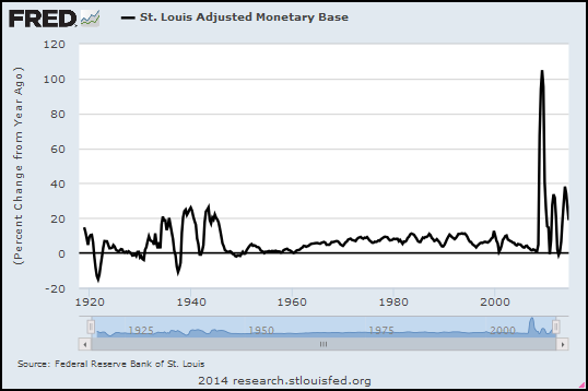
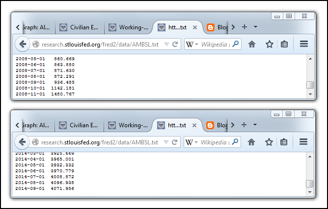
Graph #1: Percent Change, Base Money, Monthly Data: 2004-08-01 to 2014-08-01
August 2008 marks the end of relatively tame money growth. September 2008 marks the start of aggressive money growth. September 2014 marks a full six years of aggressive money growth. And yet two different price indexes both show that inflation since September 2008 has been milder than it was in the period before that date:

Graph #2: CPI (blue) and PCE (red) Inflation Measures, Monthly, 2004-08-01 to 2014-08-01
We've had less inflation since QE began than we had in the years before QE. And we want the threat of inflation to be gone. Doesn't that count for something?

Not much. No.

Tuesday, October 7, 2014

"He seemed completely unable to grasp that I was talking about the conventional use of words..."


From Names Are Conventional at La Bocca della Verità:
Is Pluto a planet?

Pluto itself simply is what it is, and does what it does, regardless of what we call it. The question "Is Pluto really a planet?" is confused: The real question is, "Is our classification system more helpful to us if we classify Pluto as a planet, or if we do not?"

Astronomers recently decided that the right answer is: "Not." Given I am not an astronomer, I trust them, and suspect they made the right decision. But the question is completely different from one such as, "Does Pluto have an iron core?" or "What is the period of Pluto's orbit of the sun?" The latter two questions are about Pluto; the former question is about how we want to structure our language to make it the most useful to us.
 
Is this about the economy? Sure, because we talk about the economy, too.

Recommended reading.

Monday, October 6, 2014

Stiglitz: "Any theory of deep downturns has to answer these questions"


From NBER, from the free teaser page that wants $5 for a PDF...

From the abstract (I presume) of Reconstructing Macroeconomic Theory to Manage Economic Policy by Joseph E. Stiglitz (NBER Working Paper No. 20517):
The paper argues that any theory of deep downturns has to answer these questions: What is the source of the disturbances? Why do seemingly small shocks have such large effects? Why do deep downturns last so long? Why is there such persistence, when we have the same human, physical, and natural resources today as we had before the crisis?

Gotcha covered, Joe.

  •   What is the source of the disturbances?

Financial cost.

  •   Why do seemingly small shocks have such large effects?

Debt accumulates slowly, and the cost of accumulated debt grows gradually.


As the rising cost becomes a problem, people compensate by increasing the amount they borrow. So, for a long time, the growing debt seems to have no harmful effects at all. Then one day, a straw breaks the camel's back. When that happens, the full weight of accumulated debt becomes a problem, and large effects follow from the seemingly small shock.

  •   Why do deep downturns last so long? Why is there such persistence, when we have the same human, physical, and natural resources today as we had before the crisis?

We have the same human, physical, and natural resources now as we had before the crisis. We have very nearly the same debt, also. Recommend a policy focused on reducing financial cost by reducing the accumulation of debt, and people will find a million reasons why it cannot and should not be done.

Our deep downturn could have been brought to an end quickly if a conscious effort had been made to reduce debt by a significant amount -- cut in half, say. But since we insist on letting the problem resolve itself, the downturn could last twenty years or more.

Sunday, October 5, 2014

Employment


Unemployment has been awful since the crisis. Things are getting better now, at least by some accounts. But it's easy to doubt such accounts, because demographic changes pull the rug out from under them. Or they seem to, anyway. It's all very confusing.

So here's a simple look at "employment" -- the number of workers in our economy. Instead of just raw numbers, I'm looking at the percent change in employment. I'm using quarterly data, not monthly, to make the graph less jiggy and easier to read:

Graph #1: Percent Change in the Total Employment
The trend for the past 30 years has been downhill -- from about one percent, to about half a percent. That is, from 4% annual job growth, to 2%. Now, I'm not averaging the recession years into this eyeball estimate. I'm looking at the typical growing economy. The trend of the good years has been downhill for 30 years.

And if you look at the trend line I threw in there, it looks like employment since mid-2010 has been right on trend. Maybe a pixel or two above trend. So I have to say it's not Obama or the Crisis or George W. Bush alone that is the source of the problem. I have to say the problem goes back at least to the 1980s. That means Reagan, and Bush the Father, and Bill Clinton are also part of the problem.

But I don't like to blame people. I like to blame policies. What I usually say (and I stand by it now) is that the problem goes back probably another 20 years before the 1980s. What that means is the problem is not unemployment.

The problem is Problem X. What we see on the graph -- declining employment since the 1980s -- was a "solution" to Problem X.

Is declining employment a problem? Well, sure. But it's not the problem. Declining employment was a solution to the problem. So our solution is a problem, yes. But again, it's not the problem. I hope this is making sense to you. I don't know how to say it any better.

Do I think I know what Problem X is? Of course: Excessive debt. Excessive finance. Financial "deepening". These are all the same. But don't think the problem started with Obama, or with Bush the Younger, or Clinton, or Bush the Elder, or even with Reagan. It would be more accurate to say the problem was already a problem the last time Lee Harvey Oswald fired his rifle.


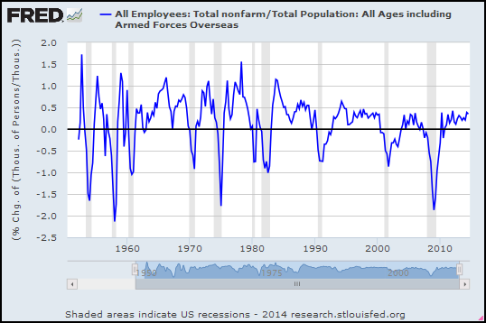
I have to say the problem goes back at least to the 1980s. But then, doubt recurs. Demographic changes come back to haunt me. So I took the total number of employees and divided it by the total population, to get the working share of population, and looked at the percent change in that. Again, quarterly:

Graph #2: Total Employment Relative to Total Population, Percent Change
As with Graph #1, #2 shows moderation for the last 30 years. Moderation and decline. Again, my trend line shows the trend of the growing economy and ignores the big, sub-zero Vee shapes associated with recession and recovery.

The trend is consistent, too. Granted, I just sketched in a straight line. But a lot of jiggles cling to that trend, in the 1980s and again in the 1990s and again in the 2000s. In comparison to this trend line, job growth for the past three years has been good (odd as that is to say). If this trend line is right, employment is well above the trend of the last 30 years. Clearly it is the last 30 years for which unemployment has been a problem, not the last three.


I found a quarterly, seasonally adjusted dataset at FRED for Working Age Population: Age 15 and Over for the United States. Starts at 1955. Maybe that's a better context than the whole U.S. population?

The Working Age Population series counts persons... The Employment series counts thousands of persons... I'll multiply the Employment number by 1000 to convert it to persons so the units match. I probably don't need to do that if we're looking at percent change numbers. But what the heck.

Again, a look at percent change:

Graph #3: Total Employment Relative to Working Age Population, Percent Change
I still say it looks like 30 years downhill. And that's for the good years.


For the Working Age Population data, FRED wants the source cited:
Working Age Population: Aged 15 and Over: All Persons for the United States©
OECD descriptor ID: LFWATTTT
OECD unit ID: STSA
OECD country ID: USA

All OECD data should be cited as follows: OECD, "Main Economic Indicators - complete database", Main Economic Indicators (database),http://dx.doi.org/10.1787/data-00052-en (Accessed on date)
Copyright, 2014, OECD. Reprinted with permission.
Source: Organisation for Economic Co-operation and Development