Friday, February 28, 2014
Thursday, February 27, 2014
 (and quoted here, too)
From David Warsh at Economic Principals: That Fateful Year, quoted by Gavin Kennedy at Adam Smith's Lost Legacy:
And at some point, I finally I realized who it was Martin so persistently reminded me. Not David Graeber, the prolix London anthropologist whose book Debt: The First 5000 Years helped inspire the Occupy Wall Street movement. Like him, Martin attaches inordinate significance to a chicken-and-egg theory of the primordial ancient origins of credit. The two are convinced that no barter economy ever existed, that symbolic money, or at least ledger debt, preceded trade. Whatever.
File that under best put-downs.
Wednesday, February 26, 2014
Among the "exponential patterns" at Bing Images...
 |
| http://easybiotechengg.blogspot.com/2013/05/microbial-growth-kinetics.html |
Notes from the old computer:
In Essays in Persuasion Keynes touched on the ideas of Professor Commons. Commons described three economic epochs--the Era of Scarcity, the Era of Abundance, and the Era of Stabilization. The era of scarcity, Keynes notes, was "the normal economic state of the world up to (say) the fifteenth or sixteenth century". The era of abundance occupied the seventeenth and eighteenth centuries and "culminated gloriously in the victories of laissez-faire". And in 1925 Keynes wrote that "we are now entering" the era of stabilization, identifying Professor Commons as "one of the first to recognize" it.
The era of scarcity was characterized by a minimum of individual liberty and a maximum of control by governmental coersion. The era of abundance was characterized by a maximum of individual liberty and a minimum of coercive control. The era of stabilization is characterized by "a diminution of individual liberty" brought about "mainly by economic sanctions through concerted action" [Keynes quoting Commons].
The era of scarcity was characterized by a minimum of individual liberty and a maximum of control by governmental coersion. The era of abundance was characterized by a maximum of individual liberty and a minimum of coercive control. The era of stabilization is characterized by "a diminution of individual liberty" brought about "mainly by economic sanctions through concerted action" [Keynes quoting Commons].
Two additional notes from that file:
"Concerted action" refers to groups and organizations--"corporations, unions, and other collective movements." Today we use the phrase "special interest groups" to refer to these sponsors of collective action.
In the 1930s Walter Lippmann wrote, "Men are asked to choose between security and liberty." [The Good Society, Introduction]
See also my prior post on Professor Commons.
Tuesday, February 25, 2014
1960? 1947?
At MacroMania, in a post titled 2008, David Andolfatto writes:
And so, it was the Lehman-AIG event that brought all financial firms under heightened suspicion--and it was this event that drove the financial crisis from September 2008 and onwards.
We all know how the Fed reacted at the time, and since then. The interesting question here is what the Fed might have done differently in the time leading up to the start of the crisis in 2007 and beyond?
David adds, "It is important to answer this question, I think, in the context of policy making that is constrained to operate with the use real-time data (that is frequently subject to significant revisions as time unfolds)."
Fair enough. But let's not go back to the crisis of 2007, nor the few months before that crisis. Let's go back as far as we can -- as far back as we can trust the data.
Monday, February 24, 2014
Before we solve the problem...
David Glasner is an economist. I am not. He did good, though: I understood about half of his What Does “Keynesian” Mean?. I lost it in the second half. But I got to his last paragraph, and I think I understood that one:
If there is widespread unemployment, it may indeed be that wages are too high, and that a reduction in wages would restore equilibrium. But there is no general presumption that unemployment will be cured by a reduction in wages. Unemployment may be the result of a more general dysfunction in which all prices are away from their equilibrium levels, in which case no adjustment of the wage would solve the problem, so that there is no presumption that the current wage exceeds the full-equilibrium wage.
Glasner says unemployment may be part of a larger problem -- "a more general dysfunction". That's important. It means we can't fix the problem with a jobs program, for example, or by printing so much money that NGDP increases at a 5% annual rate.
What it means is, we have to stop and figure out what this "more general dysfunction" is. Figure out what the problem is. Go back to square one and work it out. I don't think Glasner quite says that, but how else are we going to figure out what the underlying problem is?
Sunday, February 23, 2014
Ryan Avent's Meme of Troubles
"The productivity puzzle that began in the 1970s persists..." writes R.A. at The Economist. I like that because it takes us back to the 1970s. It takes the problem back to the 1970s. That's important. If we have a problem that started in the 1970s, we can't fix it by looking at what happened since 2008, or in the 2000s, or even in the 1980s. We have to look at the 1970s, when the problem developed. We have to look back before the 1970s, when the problem was developing and we hadn't yet noticed.
"...thanks to the apparent fizzle in productivity growth since the internet boomlet of 1996-2004..." R.A. adds, as if we all know it was the internet that temporarily solved the problem. Nice to know that, isn't it? It's nice to know things. Too bad we know all this before we even start investigating the problem. Eh, human nature: Shoot first, ask questions later.
"...and despite what looks to many like an ongoing acceleration in technological discovery." R.A. concludes his thought by pointing out something that ought to invalidate the "internet boomlet" explanation. He doesn't pursue that, but instead goes back to puzzles, and fleshes out a whole list:
There are puzzles of wage stagnation and falling labour-force participation. There are savings glut puzzles and secular stagnation puzzles. The common thread linking the puzzles is that they almost always mean trouble of one sort or another. Many stories have been presented to explain some of these phenomena (and others, as well, like rising inequality and the striking emergence of jobless recoveries)...
R.A. wants to "tie these stories together into ... a broader theory of troubles."
"The immediate motivation for the argument presented here," he writes, "is work done on the diverging fortunes of the British and American economies over the past six years." Over the past six years, he says. So much for the 1970s.
I don't have to read any more to know that R.A. is not attempting to discover the root of the problem. I already know he is looking only at results of what has become a 40-year-old problem. I'm sure he will make a good story of it, and I'm sure he will convince some people. But it will be all an investigation of results, and at best an attempt to solve results rather than to uncover and solve the problem.

R.A. then begins to make the key points of his argument. "Since the early 1980s, labour markets have polarised or 'hollowed out'", he writes. And "Since the early 1980s, polarisation has occurred almost entirely during recessions."
But these are the early responses to the problem that
Then he makes a most interesting observation:
The jobless recoveries of the past generation have been characterised by a change in the cyclical behaviour of productivity.
Prior to the mid-1980s both output and productivity growth tended to fall relative to trend in recessions and rise relative to trend in expansions. Beginning with the recovery from the 1981-2 recession, however, the behaviour of productivity flipped. It has since risen relative to trend in recessions and fallen relative to trend in expansions.
Prior to the mid-1980s both output and productivity growth tended to fall relative to trend in recessions and rise relative to trend in expansions. Beginning with the recovery from the 1981-2 recession, however, the behaviour of productivity flipped. It has since risen relative to trend in recessions and fallen relative to trend in expansions.
 |
| Graph #1 |
Quite a coincidence. Or rather, quite a striking chronological similarity.
The things that were different since 1981, including the cyclical behavior of productivity and the trend of interest rates, must be considered together, and considered as a description of the key change that occurred in 1981 when Paul Volcker broke the forces driving interest rates.
I do not identify the key change. I only emphasize that we must identify it. But Ryan Avent does neither. He moves instead to conclusion:
Taken together, these observations imply that in the presence of moderate inflation, real wages will be more flexible and productivity will flip back to falling, rather than rising, amid weak demand. That brings us back to the motivating example of the Britain versus America comparison, where that implication seems to have verified.
Verified, he says.
Me? I'm talking about gathering up things that changed in 1981 and considering them. I'm talking about pushing the envelope back to 1960 to seek preliminary indications of the cause of the "productivity puzzle that began in the 1970s".
R.A.? He's confirming things already. He's verifying things by looking over "the past six years" and by plucking observations out of the mid-1980s when people were already responding to the puzzle of the 1970s and to the fine handicraft of Paul Volcker.
Verified? Don't even think about it.
Avent then draws "further lessons from this". I love it. Jump to conclusions, then build on them right away. Don't give people time to mull them over. Build on them, tie them into your story, interpret them in the way that furthers your story. Make them part of your meme.
Avent:
These facts describe a particular relationship between technological change and macroeconomic policy. Low inflation in the era after the Volcker recessions significantly reduced the flexibility of real wages. As a result, employers faced pressure to raise employee productivity at times of weak demand, in order to reduce the effective real wage of existing workers.
See? I told you it'd be a good story. R.A. goes on from there, to build what even he calls a story. "The key dynamic in this story," he writes, "is steady improvement in technological progress."
And it is a well-told tale. Everything fits. Everything comes together and it all makes sense. Why? Because in the economy, everything affects everything and it is all related. It is not difficult to pick a starting point and develop a story in which everything is an outgrowth of your particular starting-point. It's not difficult, at all. That's how we get so many contradictory versions of how the economy works and what's wrong with it.
It's like solving a math problem. If you start in the wrong place, you can do everything else right and still get the wrong answer. Ryan Avent starts in the wrong place. He doesn't go back to the time before the problem first arose.
The problem that arose in the 1960s was the growing accumulation of private debt. Growing debt increased costs for those who owed it and increased incomes for those who owned it. These initial costs stand as the force underlying the rise of the Great Inflation in the mid-1960s.
But the economy was still good in those years. Not a lot of "toxic assets" back then. The owners of debt made reliable income from it. It was more appealing than having to work for your income, evidently, as finance grew far faster than output:
 |
| Graph #2: Total Financial Assets of Financial Business (blue) and GDP (red) See also Total Financial Assets of Financial Business as a Multiple of GDP at FRED |
 |
| Graph #3: Doug Henwood's Graph |
Income was redirected away from wages, and into the financial sector. This is clearly evidenced in corporate cost trends:
+(2).png) |
| Graph #4: Employee Compensation (blue) and Business Interest Cost (red) as Percent of their Sum |
By the 1980s policies were being put in place -- supply side policies, intended to boost supply side income. These policies worked largely by changing the distribution of income. Today's income inequality is a result of policies designed to boost economic growth by creating supply side advantages.
But the original problem goes back to the 1950s and 1960s, the gradual, relentless increase of financial income relative to wages and productive-sector profit.
Saturday, February 22, 2014
They think it doesn't work, but they use it anyway.
The other day I wrote:
I assume Sethi, like everybody else, bases his determination on economic conditions. You know, the Phillips tradeoff: inflation and unemployment. The great, sad irony is that we continue to rely on the Phillips tradeoff, even though the Phillips curve has had the obligatory funeral.
I was a little nervous about that. Not because I said Sethi relies on the Phillips tradeoff, no. That's a specific statement, easily corrected if I got it wrong. I was nervous about the general statement, my claim that everybody relies on the Phillips tradeoff. I'm nervous because the statement is based on my impression of things. I like to have something stronger behind what I say.
So I was glad to read JW Mason write:
... Perhaps more importantly, this is a rejection not just as of MMT but of almost all policy-oriented macroeconomics, mainstream and heterodox. Whether you're reading David Romer or Wendy Carlin or Lance Taylor, you're going to find a Phillips curve that relates inflation to current output.
In other words, in almost all policy-oriented macro, you find the Phillips relation. Wow, was I happy to read that!
Mason again:
MMT has exactly the same theory of inflation as orthodox macro: High or rising inflation is the result of output above potential, disinflation or deflation the result of output below potential. In other words, MMT is consistent with a standard Phillips curve of the same kind Palley (and almost everybody else) uses.
Romer and Carlin and Taylor and MMT and Palley and almost everybody else: They all rely on the Phillips curve.
So I feel a little better about my impression of things.
From Mark Thoma
Like Robert Waldmann, I have always taught that the Phillips curve was initially promoted as a permanent tradeoff between inflation and unemployment. It was thought to be a menu of choices that allowed most any unemployment rate to be achieved so long as we were willing to accept the required inflation rate...
However, the story goes, Milton Friedman argued this was incorrect in his 1968 presidential address to the AEA. Estimates of the Phillips curve that produced stable looking relationships were based upon data from time periods when inflation expectations were stable and unchanging. Friedman warned that if policymakers tried to exploit this relationship and inflation expectations changed, the Phillips curve would shift in a way that would give policymakers the inflation they were after, but the unemployment rate would be unchanged. There would be costs (higher inflation), but not benefits (lower unemployment).
When subsequent data appeared to validate Friedman's prediction, the New Classical, rational expectations, microfoundations view of the world began to gain credibility over the old Keynesian model...
That was the beginning of the end of the Keynesian consensus.
It was also the end of the Phillips Curve. Except, it wasn't. The Curve got split in two: the short run, and the long run. Like wise men, everybody rejected the long version. But everybody still relies on the short version. In other words: They think it doesn't work, but they use it anyway.
Here -- The CBO relies on the Phillips tradeoff when they figure Potential output:
CBO’s estimate of potential output is based on ... a relationship known as Okun’s law.
According to that relationship, actual output exceeds its potential level when the rate of unemployment is below the “natural” rate of unemployment...
For the natural rate of unemployment, CBO uses... NAIRU [which] derives from an estimated relationship known as a Phillips curve...
Everything seems to depend on the difference between short-run and long-run. So I ask: What happens in those precious moments between the short run and the long?
In the short run, they increase the money rapidly, catching us by surprise, and so we buy more and produce more because we have more money without knowing it, and unemployment goes down. That's the short run.
In the long run we figure it all out, and we swear we won't get fooled again. We quit buying more and we quit producing more because we know about the money now. And unemployment goes back up.
Is that really what Milton Friedman said?
Friday, February 21, 2014
Economic forces be damned
You can think of this post as a follow-up to my Queen of the Prom and my Loosey Goosey and the Four-Letter Word and my best criticism of Scott Sumner's analysis
"Loose" and "tight" are words one uses to evaluate monetary policy, which affects inflation and unemployment, which are captured in the Phillips Curve tradeoff.
That's all. I just wanted to make the point that Sumner's twiddling with loose and tight is an attempt to get at the workings of inflation and growth, which means his twiddlings are related to the Phillips trade-off.
Sumner's focus on loose and tight differs from everybody else's by way of the "relative to". Everybody else seems to think in terms of loose or tight relative to how things were before. Sumner seems to think of it relative to what the result looks like to Sumner. He says NGDP is not increasing at a decent rate, so money must be tight.
I may have to apologize for saying this, but Sumner's view is the most simplistic bullshit I've ever seen. That's not how the economy works.
How much money growth does Scott Sumner want? There is no limit, I guess, if what we've been doing isn't enough for him. Sumner wants whatever it takes to push NGDP growth up to 5% annual. But the economy doesn't work that way.
It shouldn't be up to an old hippie like me to explain this to a hip young economist like Sumner: The economy doesn't work that way. You can't just keep pouring in money forever in 35 or 40% bursts and getting out one or two percent inflation. Eventually -- if the economy comes back to life -- there'll be inflationary hell to pay for that kind of shortsightedness. And if the economy never comes back to life, well, that's all she wrote for the U.S. of A.
According to Sumner, people other than Sumner say that money is easy when interest rates are low, and tight when interest rates are high.
Today we might think of 5% as a high rate of interest. Rates two to three times that level might have been called high in decades not long past. In those times, 5% would have been called a low rate.
What number is a high rate? What number is low? It varies, obviously, as time goes by.
In this sense, Sumner has to be right: Low as interest rates are these days, they are too high to give us a growing economy. Remarkably, Paul Krugman seems to agree with Sumner on this. Krugman spends a lot of time talking about the Zero Lower Bound as something that prevents rates from being as low as they need to be to give us a growing economy.
Sumner seems to work backward from the "no growth" economy to an "interest rates are too high" conclusion, and he claims that money must be tight, because the economy is not growing. This is where the simplistic hits the fan: If the economy's not growing, money must be tight.
Does Sumner say why the economy isn't growing? Other than his obsessive claim that money is tight, I don't think he does. I admit I don't read him often, but I don't think he does.
And yet, Scott Sumner is right: Money is not easy enough to grow the economy. Money isn't easy enough even to inflate the economy. And if Sumner is right about this, then something changed. Something must have changed. Something in the economy is different than before.
If this is true, then the appropriate solution is to figure out what changed, and fix it. But Sumner doesn't do that. He opts for a direct, simplistic solution.
Economic forces be damned. That's what he is saying.
"Loose" and "tight" are words one uses to evaluate monetary policy, which affects inflation and unemployment, which are captured in the Phillips Curve tradeoff.
That's all. I just wanted to make the point that Sumner's twiddling with loose and tight is an attempt to get at the workings of inflation and growth, which means his twiddlings are related to the Phillips trade-off.
Sumner's focus on loose and tight differs from everybody else's by way of the "relative to". Everybody else seems to think in terms of loose or tight relative to how things were before. Sumner seems to think of it relative to what the result looks like to Sumner. He says NGDP is not increasing at a decent rate, so money must be tight.
I may have to apologize for saying this, but Sumner's view is the most simplistic bullshit I've ever seen. That's not how the economy works.
 |
| Graph #1: Change in the Monetary Base, Different Since the Great Recession |
How much money growth does Scott Sumner want? There is no limit, I guess, if what we've been doing isn't enough for him. Sumner wants whatever it takes to push NGDP growth up to 5% annual. But the economy doesn't work that way.
It shouldn't be up to an old hippie like me to explain this to a hip young economist like Sumner: The economy doesn't work that way. You can't just keep pouring in money forever in 35 or 40% bursts and getting out one or two percent inflation. Eventually -- if the economy comes back to life -- there'll be inflationary hell to pay for that kind of shortsightedness. And if the economy never comes back to life, well, that's all she wrote for the U.S. of A.
According to Sumner, people other than Sumner say that money is easy when interest rates are low, and tight when interest rates are high.
Today we might think of 5% as a high rate of interest. Rates two to three times that level might have been called high in decades not long past. In those times, 5% would have been called a low rate.
What number is a high rate? What number is low? It varies, obviously, as time goes by.
In this sense, Sumner has to be right: Low as interest rates are these days, they are too high to give us a growing economy. Remarkably, Paul Krugman seems to agree with Sumner on this. Krugman spends a lot of time talking about the Zero Lower Bound as something that prevents rates from being as low as they need to be to give us a growing economy.
Sumner seems to work backward from the "no growth" economy to an "interest rates are too high" conclusion, and he claims that money must be tight, because the economy is not growing. This is where the simplistic hits the fan: If the economy's not growing, money must be tight.
Does Sumner say why the economy isn't growing? Other than his obsessive claim that money is tight, I don't think he does. I admit I don't read him often, but I don't think he does.
And yet, Scott Sumner is right: Money is not easy enough to grow the economy. Money isn't easy enough even to inflate the economy. And if Sumner is right about this, then something changed. Something must have changed. Something in the economy is different than before.
If this is true, then the appropriate solution is to figure out what changed, and fix it. But Sumner doesn't do that. He opts for a direct, simplistic solution.
Economic forces be damned. That's what he is saying.
Thursday, February 20, 2014
It's not the same old same old
Lars Christensen writes There is nothing “unconventional” about money base control. I don't agree:
|
| Graph #1: Change in the Monetary Base, Different Since the Great Recession |
Wednesday, February 19, 2014
Second thoughts on Rajiv Sethi's Personal Reserve Accounts
As things stand now, Treasury gets the money -- the profit earned by the Federal Reserve. That money goes to Treasury. Under Rajiv Sethi's plan that money goes instead into personal accounts for everybody with a social security card. For the year 2012, that number was $88.4 billion. Divvy that up among 312.8 million people in the U.S. in 2012, and people get about 283 dollars each. Less than we got from George W. Bush back in 2008, the stimulus check everybody supposedly saved, maybe you remember.
If people let that money sit in their accounts at the Fed, it does nothing for the economy. If people spend the money, it boosts the economy some. But the money didn't come from nowhere. It's the money Treasury didn't get. If the government spending doesn't change, then the economy gets a boost when people spend the money.
But if the government cuts back its spending by $88.4 billion so as not to increase the deficit, this cutback undermines any boost there might have been from the people spending that money.
Tuesday, February 18, 2014
The Payments System and Monetary Transmission: One Little Thing
Following up on Rajiv Sethi's wonderful post that I looked at on Sunday. If everybody had bank accounts at the Federal Reserve, Sethi writes,
profits accruing to the Fed as a result of its open market operations could then be used to credit these accounts instead of being transferred to the Treasury. But these credits should not be immediately available for withdrawal: they should be released in increments if and when monetary easing is called for.
Sethi shows a bit of caution there. Probably wise. But I don't like his method of determining if and when monetary easing is called for.
Well, he doesn't specify it in the post. I assume Sethi, like everybody else, bases his determination on economic conditions. You know, the Phillips tradeoff: inflation and unemployment. The great, sad irony is that we continue to rely on the Phillips tradeoff, even though the Phillips curve has had the obligatory funeral.
Sethi is right to say we need better methods of monetary transmission. What he neglects to say is that we also need a better indication of "if and when" easing is called for. We need a better indicator of monetary conditions.
We need to look at the ratio of dollars that must be paid back, relative to dollars available to use for those payments. In other words, dollars of debt relative to dollars that can be used to pay down debt without creating new debt in the process. For it is only from the stock of existing dollars that money can be taken to finally reduce debt.
What is needed most is not to release the Personal Reserve Account funds "in increments if and when monetary easing is called for" but to look at the ratio of debt per dollar to determine what monetary conditions really are, and to drive that ratio toward its optimal range by "releasing" funds and at the same time deconstructing incentives to borrow.
Fail to do this, and we fail to take full advantage of Sethi's money transmission mechanism. Fail, and we fail to correct the imbalance between the level of accumulated debt and the quantity of money available for settlement of debt.
Monday, February 17, 2014
What's my share?
Okay. Rajiv says everybody should have a bank account at the Fed, and the Fed should distribute its profits equally across all those bank accounts.
How much is that, per person?
| Graph #1: "Interest on Federal Reserve Notes" from the 2012 Annual Report of the Federal Reserve, Table 11. The blue line shows the years 1996-98 when Interest on Federal Reserve Notes fell briefly to zero and "Statutory Transfers" made up the difference. These transfers were "made under section 7 of the Federal Reserve Act for 1996 and 1997". View or Download Table 11 from the 2012 Annual Report (PDF, 3 pages) |
Well, at least it's more than $3.19 apiece.
Seriously, though... The purpose of the Fed profit redistribution is not to serve as a Basic Income Guarantee. The purpose is to correct a monetary imbalance -- the imbalance between circulating money and private debt. That's what makes the idea so interesting.
Sunday, February 16, 2014
Rajiv Sethi: The Payments System and Monetary Transmission
"This is an idea that's long overdue," says Rajiv Sethi. "Allowing individuals to hold accounts at the Fed would result in a payments system that is insulated from banking crises."
Sethi lists several features of such a system, features I'm quite sure you like. "But the greatest benefit of such a policy would lie elsewhere," he says, "in providing the Fed with a vastly superior monetary transmission mechanism." He writes:
Any profits accruing to the Fed as a result of its open market operations could then be used to credit these accounts instead of being transferred to the Treasury.
"It's helicopter money," says Nick Rowe in comments.
"That's exactly what it is Nick," Rajiv Sethi says.
It is a way to put money into the economy without adding debt to the economy. It is exactly what we need. It is a far, far better idea than, say, letting the Fed fund a lottery (which is the best I could come up with). It is a way to reduce the debt-per-dollar ratio and restore vigor to our economy.
"The main advantage of such an approach is that it directly eases debtor balance sheets," Sethi says. "In contrast, monetary policy as currently practiced targets creditor balance sheets." Yes! This is precisely what I was trying to convey here:
The Federal Reserve created "money from nothing"... and used it to buy up "toxic assets" in order to reduce "risk" in the financial sector... It had to be done. But look what it did: It took risky assets out of the economy, and left the risky liabilities to fester.
and again here:
The Fed buys the IOU from my lender. The lender gets cash. And I get to make the same payments I made before, except now I pay somebody else. That really doesn't do much for me. It doesn't do much for the economy, either.
Purchasing assets removes those assets from the economy, replacing them with money. But the liabilities remain as they were: draining income, depressing demand, hindering economic growth.
We have to deal with problem liabilities, not just problem assets. We have to ease things for debtors, not just for creditors. Otherwise, the economy never heals.
Saturday, February 15, 2014
Been there, done that
James Kwak explains Why We Have a Debt Problem.
First seven words: "So, we have eleven aircraft carrier groups."
1. Kwak isn't talking about the debt problem. He's talking about public debt.That's not the debt problem.
2. Kwak is talking about military spending. He's gonna want to cut military spending. That's the red line here:
 |
| Graph #1: Total (blue) and Military (red) expenditures of the Federal Government |
 |
| Graph #2: Military Expenditures as a Percent of Total Federal Expenditures |
Friday, February 14, 2014
It's always on the house at Mason's Bar and Grill
At the Slack Wire: JW Mason's Don't Start from the Coin. Mason writes:
To understand the monetary nature of modern economies, you need to begin with the credit system, that is, the network of money obligations. Where we want to start from is a world of IOUs. Suppose the only means of payment is a promise to pay. Suppose it's not only possible for me to tell the bartender at the end of the night, I'll pay you later, suppose there's nothing else I can tell him -- there's no cash register at the bar, just a box where my tab goes. Money still exists in this system, but it is only a money of account... If you give something to me, or do something for me, the only thing I can pay you with now is a promise to pay you later.
That's a little weird, isn't it? Every day at opening I tell the buxom barkeep, "Put it on my tab." And every night, stumbling out, I tell her "I'll pay you tomorrow." [1]
Let's take Mason's "bartender" example as a starting point in his "begin with the credit system" approach. Let's see what we have to add to it, so it makes sense.
There is no settlement of money obligations in Mason's Bar. Right off the top, I'd say we have to add the cash register and some means of actual payment. But hey, let's see where Mason takes us.
"Debts in this system are eventually settled," he writes. "As Schumpeter says, they're settled by netting my IOUs to you from your IOUs to me." Reminds me of the story about the $100 bill.
By the end of that paragraph, JW Mason is reiterating the "clearinghouse" function of today's central bank:
The longer the chain [of IOUs], the more important it is for their to be some setting where all the various debts are toted up and canceled out.
Mason points out that this same function was served by the great fairs of Medieval Europe:
During their normal dealings, merchants paid each other with bills of exchange, essentially IOUs that could be transferred to third parties. Merchants would pay suppliers by transferring (with their own endorsement) bills from their customers. Then periodically, merchant houses would send representatives to Champagne or wherever, where the various bills could be presented for payment. Almost all the obligations would end up being offsetting.
During their normal dealings, merchants accumulated IOUs. At the fairs, they settled them. Okay, I can see that. Mason quotes Fernand Braudel:
The fairs were effectively a settling of accounts, in which debts met and cancelled each other out, melting like snow in the sun: such were the miracles of scontro, compensation. A hundred thousand or so "ecus d'or en or" - that is real coins - might at the clearing-house of Lyons settle business worth millions; all the more so as a good part of the remaining debts would be settled either by a promise of payment on another exchange (a bill of exchange) or by carrying over payment until the next fair: this was the deposito which was usually paid for at 10% a year (2.5% for three months).
Mason likes this. He emphasizes that
a "good part" of the net obligations remaining at the end of the fair were simply carried over to the next fair.
And he moves to conclusion:
I think it would be helpful if we replaced truck-and-barter with something like these medieval fairs, when we imagine the original economic situation.
I don't understand. What does Mason mean, when we imagine the original economic situation? He seems to be suggesting that how we think about money today depends on how we think about money in "the original economic situation". That's absurd. It's more like the other way around.
Apart from that conclusion, Mason emphasizes the importance of settlement of money obligations. It seems to be the mutual swap of IOUs that satisfies his desire to understand "the monetary nature of modern economies".
And the way things are yet today, with still so many IOU dollars per settlement dollar, Mason's focus on IOUs is understandable. But then, with so many IOU dollars per settlement dollar, it is quite clearly not true that "As Schumpeter says, they're settled by netting my IOUs to you from your IOUs to me." Our world is more like Mason's Bar, where settlement never happens.
I have a different conclusion.
I think it's intuitive that, if we owe each other $100, it should be quite easy to cancel those debts. I don't think this is any great insight. I think a focus on the "settlement" service provided by fairs (or by central banks) is like blinders that keep us from seeing more significant details.
In the Middle Ages, millions of dollars of debts could be settled by a hundred thousand ecus d'or. Today, millions of dollars in promises to pay can be settled by a hundred thousand in settlement money. It's the same story as in the Middle Ages.
The story is that, while much of our debt can be settled by mutual swap and the "melting like snow", not all of it can be settled that way.
Anyway, it's important to note that it took real money to settle things, even in the Middle Ages. Mason wants us to start at the bar that has no cash register and no way to pay for our drinks. But at the end of the day, at the end of the fair, when Judgement Day comes, when it's time to settle up, you need more than just a box where your tab goes. You need the cash register. And you need something more than a promise to pay your bill later. You need money to pay your bill. You need money for settlement.
Mason says "a 'good part' of the net obligations remaining at the end of the fair were simply carried over to the next fair." But those obligations were not "simply" carried over. They were carried at 10%.
And that's just one year. Imagine a society where policy tells us it is okay to accumulate our carried-over obligations. Then most of this year's carry-over is still with us when we add next year's carry. And the year after that, and the year after that, and the year after that. Keep it up for sixty years, and this is what you get:
 |
| Graph #1: How much debt we have, per dollar of settlement money we have |
Mason wants us to think not in terms of truck-and-barter, but in terms of the Medieval fair. I want us to think in terms of the ultimate settlement medium. If most of our debt melts away like snow, great. But what about the rest? It takes money to settle that debt. If not settled, it still takes ten percent.
The IOUs that easily melt away by mutual swap are not the problem. The unsettled debts that accumulate are the problem. Thinking of the economy in terms of "melt like snow" doesn't deal with the problem. To deal with the problem, we need money for settlement.
I followed Mason's Braudel link. Braudel writes of "the old fairs at Champagne" at their peak, around 1260. And of later fairs at Piacenza, and the Genoese clearing-house. Braudel writes:
All good things come to an end however, even the ingenious and profitable Genoese clearing-house. It could only function if sufficient quantities of American silver reached Genoa. When the silver supplies began to dry up in 1610 or so, the whole structure was threatened.
The clearing-house could only function if there were sufficient quantities of silver, Braudel says.
Our debt, the whole house of cards, rests on a little bit of settlement money. It's this settlement money we have to add so Mason's story can make sense. But settlement money is the part JW Mason seems to want to do without.
Try to make sense of things without that money, and you're back at Mason's Bar.
JW Mason wants to replace "truck-and-barter" with "medieval fairs". Fine. But Braudel says medieval fairs only work if there is sufficient settlement money. Even if you "begin with the credit system" you have to end by assuring there is sufficient settlement money, or "the whole structure" is threatened.
Notes
1. I'm pretty sure Mason doesn't really mean it's always on the house at the bar he describes. He means my tab will come due sooner or later, when they open the box and tally it up and hold me accountable (i.e. "money of account"). And then I'll be stuck doing something to pay off the tab, and the question of what I won't do for money comes up for negotiation. That's probably what Mason means. But then, maybe when the time comes to pay my tab, I can just say, "the only thing I can pay you with now is a promise to pay you later."
2. Mason and Schumpeter object to "building up the analysis of money, currency, and banking" by beginning with "an analysis of a state of things in which legal-tender ‘money’ is the only means of paying and lending." Both Mason and Schumpeter prefer "to begin with the credit system".
But focusing on the one or on the other is the wrong focus. What's important is to maintain a viable balance between the quantity of credit and the quantity of the legal-tender money -- between the debt arising from credit use, and the money we use for settlement of that debt.
3. Happy Valentine's Day.
Thursday, February 13, 2014
"Get your billion back, America" ... You've seen the ad?
A billion dollars is less than $3.19 apiece.
Wednesday, February 12, 2014
Hayward is right
Off you go now, to Gene Hayward's recent post: Inflation is not a boring topic. It is a thief in the night and the root cause of rebellion around the world. Can't get more exciting than that! See here why...
Tuesday, February 11, 2014
Vintages
If you go to a FRED page like Federal Government Current Receipts (FGRECPT) you get a graph and some other stuff. If, instead of editing the graph, you look over at the sidebar, one of the items under Tools is "Vintage Series in ALFRED". If you click that from FRED's FGRECPT page, you get the ALFRED page for FGRECPT. Then you can edit it just the same as at FRED, except you can also select new or old versions of the data. New or old "vintages" they call them.
You can compare new and old vintages. For example, here are eight views of Federal government current receipts in the 1960s -- the the one that was current when I made the graph, and the first vintage from each of the previous seven years:
+vintages.png) |
| Graph #1 |
Here now are the first vintages for the most recent eight years, for Federal government current expenditures in the 1960s:
+vintages.png) |
| Graph #2 |
+vintages.png) |
| Graph #3 |
Graph #3 looks at the first vintage for each year. Graph #4 looks at every month's vintage. So, the ten most recent vintages. That takes us back before the "comprehensive revision" of mid-2013:
 |
| Graph #4: The Change First Appears in the July 2013 Vintage |
I should have known.
Monday, February 10, 2014
Don't think for a minute
 |
| Mike Kimel's Graph with Kimel's 2011 Data (upper part) and the Current 2014 Data (lower part) |
Don't think for a minute that the change in Kimel's graph is due to a "revision" of the data. There was obviously something wrong with his Federal deficit numbers from the start.
Surely you know that US economic growth was good in the 1960s -- very good, at that. It was so good, it is the kind of thing people know without stopping to look it up.
And surely you know of the "full employment budgets" and of "potential output" and of policy attempting to push output up in the 1960s by means of deficit spending.
Surely you know of these things, no?
And yet, it seems Mike Kimel overlooked those things when he made his graph. Did he stop to wonder why his numbers show balanced budgets in the 1960s?
If you read his post when it was new, didn't you wonder?
This has nothing to do with the revision of data. It has to do with paying attention to things we know, and making sure new information fits with what we know.
Hey -- Kimel's balanced budgets in the 1960s could have been correct. But then, we would have had to take something else we thought we knew, and toss it.
Sunday, February 9, 2014
Kimel's spreadsheet is a beautiful thing
Mike Kimel's spreadsheet contains a page where he pasted BEA Table 3.2. The table shows a breakdown of Federal government revenue and spending for the 1929-2010 period. Then at the far right, beyond the table, he pulls out and gathers the data on "current revenues" and "current expenses" and uses those numbers to calculate a surplus or deficit for government spending.
Where Kimel pulls out and gathers the numbers, he doesn't do it by copying and pasting. He does it by setting cells equal to values in the table. "Referencing" cells in the table, it's called.
This is kind of important. I captured part of Kimel's spreadsheet page in Zoho so you can look at it. Column C contains the BEA's breakdown of Federal receipts and expenditures. You don't have to memorize it, but you should note that the breakdown contains a lot of line items -- 46 of them, according to the numbers in Column B. In the spreadsheet, you can scroll down to see the whole list. You can press CTRL+HOME to get back to the upper left cell A1.
You can scroll to the right. To the right of Column C, I've included the first five years of the data that run from 1929 to 2010 on Kimel's sheet. The numbers in this table are numbers, not calculations.
At the top of the spreadsheet below, just down from the title "Kimel Fragment" is a white field less than an inch wide, then the letters FX in some fancy font, and then a white field about 3 inches wide. That wide white field is the "formula bar". That field displays the contents of the cell you select, and it changes as you move the cell selector.
If you move the cell selector to column D or E or F or G or H, you can see that the entries for "Current receipts" and "current tax receipts" and "Personal current taxes" and the others are actual numbers. Not calculations or formulas, I mean.
If you scroll a little more to the right you come to a blue area. (I made the background blue so I could describe it easily and you could find it easily.) Scroll a little more to the right, so you have the whole blue area on the screen.
If you move the cell selector around in the blue area, you will notice that the titles on Row 2 ("current receipts" for example) appear in the formula bar when those cells are selected. That tells you that Mike Kimel (or somebody) actually typed those words into those cells. Or maybe that they copied those words from somewhere else and pasted them into those cells.
If you move the cell selector along the left edge of the blue area, on the year values, you will notice that the year values appear in the formula bar. These numbers also were typed in, or pasted in.
That could be done differently. You could type 1929 in cell J3, and do the numbers below it just by adding 1 each time you go down a line. For example, in cell J4, where you want the value 1930, you want a value that is one more than the value in cell J3. So you could add 1 to the value in cell J3.
To do that you would select cell J4, then type an equal sign, the number 1, a plus sign, the letter J, the number 3, and then you would hit the ENTER key. (Try it if you want. You won't mess up the sheet. If you do mess it up, just refresh the page and start over. No harm done.)
When you hit ENTER the cell selector moves down a row, onto the value 1931 (which is a typed-in number). Move the cell selector up a row, onto the value 1930. Notice that in the blue area, the cell shows 1930 but in the formula bar it shows the formula that you typed in: =1+J3 .
That's why I like Zoho. It lets you use the formula bar online.
Now if you wanted to recreate the value 1931 in the next cell down, you could do it with a formula just the same way. Actually, it would be the same formula. (And now we're getting somewhere!) In cell J5 you would want the value 1 plus the value in the cell above. But you don't have to type the formula again. There's an easier way.
Move the cell selector to cell J4, where your formula is. Right-click on that cell, and select COPY from the little menu that shows up.
Select the next cell down -- cell J5 -- and press CTRL-V.
Nothing happens in the blue area. But the formula bar changes.
Do it again. Select the next cell down and look at the formula bar to see that it contains a year number. Then press CTRL-V, and the formula bar will show your formula instead.
Okay, now for the good part. Click on the next cell down, but don't release the mouse button. Instead, drag the mouse down several rows. Yes, yes, do go three or four rows off the blue area, yes!
Now press CTRL-V.
All the cells you selected get the blue background color. And, if you stayed in Column J, all the cells you selected now show year values, in sequence.
So I hope you already knew how to do that. But if you didn't, wow. You should learn. I'll help you if you want. We can do more of this spreadsheet stuff. Just not in this post.
So anyway, look at the values for "current receipts" and "current expenditures" for 1929 to 1933, in the blue area on the spreadsheet. In the blue area, there are values. But in the formula bar, there are formulas. The one for cell K3 shows =$D$3 for example.
It starts with an equal sign, just like the formula we entered to get the year values.
There are a couple dollar signs in it though. That's okay. We're not doing any more spreadsheet lessons in this post. Overlook the dollar signs in the formula. If you ignore those dollar signs, the formula looks like =D3. That means the value in cell K3 comes from cell D3. If you scrolled back over to Column D, you'd see the same value in that cell as in cell K3.
And in fact, if you changed the value in cell D3, the value in cell K3 would also change! That's pretty neat. It's a powerful feature of spreadsheets, and it's one reason people use them. I made use of that feature for this series of posts.
What I did was, I got the latest values from the BEA site, their Table 3.2 that shows current receipts and current expenditures. I added that sheet as an extra sheet in Mike Kimel's spreadsheet. And then I went into Mike Kimel's Table 3.2 and used formulas to set the "current receipts" and "current expenditures" values in Kimel's table equal to the new 2014 values.
I only had to create formulas for the 1929 values. Then I copied those formulas over to the later-year columns. Easy as that, Kimel's sheet contained the new 2014 values.
And then, because Mike Kimel did his spreadsheet the right way, using formulas that refer to to other cells, all of his numbers got updated. (I only changed "Line 1" current receipts and "Line 20" current expenditures. But those are the only numbers Kimel uses from Table 3.2. And every place he used those numbers, they got updated.)
So I made an easy change, updating Mike Kimel's data. And the prize I got for that was an updated version of his graph, as you can see below.
 |
| Graph #1: Kimel's Graph with Kimel's BEA Data |
 |
| Graph #2: Kimel's Graph with Current BEA Data |
Related Files
1. Mike Kimel's original Excel file, which he very generously sent upon my request: Tabarrok and Cowen 20110217 follow up 20110221.xls
2. Downloaded from BEA, the current (30 Jan 2014) version of Table 3.2 (for Federal spending and revenue): BEA download.xls
3. File 2 as a page in file 1, allowing me to revise Mike Kimel's graph by referencing the more recent values: Current BEA data.xls
4. For yesterday's graph of Real Private Spending in the 1960s, the Google Drive spreadsheet named A Look at Mike Kimel's Data. That's the original Excel file Kimel sent me, converted to Google Docs format. So I could look at his data for the 1960s.
Saturday, February 8, 2014
Keynes, Keynesians, and Deficits as Policy
“New Keynesianism” is a gross misnomer. The macroeconomics of people like Greg Mankiw and Paul Krugman has theoretically and methodologically a lot to do with Milton Friedman, Robert Lucas and Thomas Sargent — and very little, or next to nothing, to do with the founder of macroeconomics, John Maynard Keynes.
I have to talk about a Mike Kimel post from back in February 2011 -- his Critique of Tyler Cowen’s The Great Stagnation, by way of Alex Tabarrok’s Criticism of Keynesian Politics. You can see the post at Angry Bear or at Presimetrics. The Presimetrics link is missing Kimel's very important graph, but carries some comments by Mike Kimel that the AB post lacks.
I was introduced to Kimel's post almost three years ago by Jazzbumpa's Accidental Keynesians, and by comments on two other posts at Retirement Blues: Money Illusion Delusion and A Different Look At The Great Stagnation - Pt 2.
Back then I had two problems with Mike Kimel's post: First, his definition of the term "Keynesian". And second, his view that in the 1960s policy was (by Kimel's own definition) Keynesian.
Those problems persist.
Two Problems
Jazzbumpa's recent Republican State of Disunion: Taxes Edition links to Kimel's old post. That's why the subject comes up. Here are my problems with Kimel's post:
1. "What Keynes called for was deficits when the private sector cut back", Kimel says in a comment at Presimetrics, "and surpluses at other times". Yes, that is exactly what Keynes said. But that is not what the policymakers did, who called themselves "Keynesian" in the 1960s. The Keynesians did not think like Keynes.
2. "The fact that the government started running non-stop deficits means that by the very definition of Keynesian economics, it wasn’t following Keynesian policies," Kimel adds. He's right again -- by his definition of "Keynesian". But Kimel says the non-stop deficits started around 1967 "or 70 or 73 or thereabouts (I think 67 but I’m open to persuasion about what date the graph points to)".
That *is* what his graph shows: 1967 or '70 or '73 maybe. But as Basil points out in the first comment on the Presimetrics post, "since ~1960, the US has been running a deficit nearly nonstop."
Basil is right. Kimel disagrees, but Basil is right. The "Keynesian" policymakers of the 1960s used "full employment" budgeting, trying to push economic growth up to "potential" by stimulating the economy with deficits. The 1960s was a decade of deficits.
Not only does Mike Kimel overlook the difference between Keynes and the Keynesians. He also overlooks the policy of the 1960s. He shows a graph that says the US ran balanced budgets through most of that decade.
Hey, definitions are definitions. I can deal with that. But the discrepancy regarding the deficits of the 1960s has been eating at my brain for three years.
Mike Kimel says Tabarrok and Cowen are wrong -- "wrong that Keynesian economics hasn’t been tried, and wrong that it hasn’t worked."
I don't want to argue that point. But I did want to gripe about Kimel's definition of Keynesian economics. And I do want to reconsider Mike Kimel's 1960s.
From Kimel's post:
The following graph may look a bit odd, since it has no curve on it. But it shows something cool. If I did this correctly, the gray bars show periods when:
1. real private sector spending hit a new high and the government ran a surplus
2. real private sector spending fell below a previous high and the government ran a deficit
Keynesian governments will generally behave in that way. The turquoise bars show non-Keynesian behavior:
1. real private sector spending hit a new high and the government ran a deficit
2. real private sector spending fell below a previous high and the government ran a surplus
Here’s what it looks like:
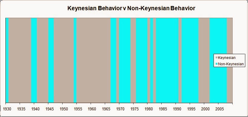 |
| Figure 1 |
The graph is wrong.
On Mike Kimel's graph, the gray areas show times when policy was Keynesian -- or, not "Keynesian", but when policy was in accord with the ideas of Keynes himself. Let's call that "Keynes-like".
On Kimel's graph, the biggest gray area is a stretch that runs from 1955 to 1967. That means policy in those years was Keynes-like. By Mike Kimel's definition, it means the private sector was growing while the government ran a surplus... or the private sector was shrinking while the government ran a deficit.
In the 1960s the economy was growing while the government ran deficits. Kimel's graph is wrong.
One of the things I know without looking is that the 1960s was a time of economic growth. Before the 1980s came along, the 1960s were often held up as the longest period of uninterrupted expansion since the Second World War.
Any chance you remember that?
Kimel's data does show that the economy was growing in the 1960s:
 |
| Graph #2: The economy was Growing in the 1960s |
And yes, Kimel's data also shows Federal revenue higher than Federal spending almost all through the 1960s:
 |
| Graph #3: Kimel's Data Shows a Budget for the Most Part in Surplus |
Those source numbers produce the large gray, Keynes-like 1960s on Mike Kimel's Figure 1. But these numbers would have produced a large turquoise area:
 |
| Graph #4: The Current Version of Kimel's Data Shows Expenditure Consistently Greater than Receipts through the 1960s. In other words, Consistent Deficits. |
Here's my problem. I know the economy was growing in the 1960s. I also know that in the 1960s, policymakers used "full employment" budgeting to stimulate further growth. They used deficits. It was policy.
It was Keynesian policy. It was not Keynes-like. There were budget deficits in the 1960s, lots of budget deficits. It was policy in the 1960s to stimulate growth by means of deficits.
There is nothing iffy about this. It was policy.
I have to say this again. The economy grew in the 1960s. Policymakers at the time thought their policy of using deficits to boost growth was working. If the economy was growing, and there were deficits, then Kimel's graph should show turquoise in the 1960s, not gray. There is a problem with his graph. I can't get around it.
 |
| Graph #5: The Federal budget "surplus or deficit" was barely above zero in 1960. It was not in balance again until 1969 under Nixon. |
 |
| Graph #6: Both the gross Federal debt, and the credit market portion of it, increase throughout the 1960s. There had to be deficits in those years. |
I have to look at Kimel's spreadsheet.
// UPDATE
Mike Kimel writes:
I would request that you immediately put up some sort of postscript indicating that a) I made the spreadsheet available to you as soon as you requested it and b) you could duplicate my results using older data, and please notify me when it is done.
He's absolutely right.
If you visit here often, you may know that I tend to split up a post into several sections. I didn't even think about it. Plus, I wrote some make-nice stuff that later got deleted. So I left a bad impression, and I apologize for that.
Not my intent, Mike. Sorry.
Even though his post is three years old, Kimel found the relevant spreadsheet and sent it to me right away. And I love the spreadsheet. It was done right, so that it was easy for me to plug in the current data. See tomorrow's post: "Kimel's spreadsheet is a beautiful thing".
Oh, and yes: I looked at the older "current expenditures" and "current receipts" at ALFRED and found data that show what Kimel showed -- budget surpluses in the 1960s. This graph:
 |
| Graph #7: Federal Budget in Surplus, except 1967 and the last bit. |
One more thing. It's not the changed data that pesters my mind. It is that Kimel used data that showed balanced Federal budgets through most of the 1960s. But the Federal debt grew in the 1960s, so I know there were deficits. Everybody knows there were deficits, I think. So I don't understand why Kimel used the data he used.
Mike, as I wrote to you this morning:
What bothers me is that I know perfectly well the Federal budget was in deficit almost without letup in the 1960s. But you selected data that (until the revision) showed the Federal budget mostly in surplus. I don't understand your choice of data.
I didn't ask for a response, because you said you are busy. Now I'm asking.
It was policy in the 1960s to use "full employment" budgets -- to use deficit spending to stimulate economic growth beyond the growth we already had at that time. As a result of that policy, there were Federal budget deficits in the 1960s.
Mike, please explain to me why you chose to use data that did not show the deficits.
Friday, February 7, 2014
MACROECONOMIC POLICY IN THE 1960s
This post provides background you'll need for tomorrow's post.
The Full Employment Budget (1)
From an undated (must be early '70s) PDF at Brookings -- The Full Employment Surplus Revisited, by Arthur M. Okun and Nancy H. Teeters. Well said:
In a period of slowdown in economic activity, the movement of the actual surplus or deficit in the federal budget must be carefully interpreted. If a shift to deficit merely reflects a slower growth of federal revenues associated with a weakening of economic activity, that shift is an automatic stabilizer bolstering demand rather than a stimulus propelling the economy.
Economists have long been concerned with the inadequacy of the actual surplus (or deficit) as a measure of fiscal impact. It fails to distinguish the budget's influence on the economy from the economy's influence on the budget. The actual surplus (or deficit) is the composite result of the budget program, as defined in terms of expenditures and tax rates, and the strength of aggregate demand. To remedy the basic defect of the actual surplus as a fiscal indicator, the concept of the full employment surplus was developed. The full employment surplus is an estimate of what the federal surplus would be if the economy were operating along the path of its potential gross national product (GNP). It is thus not affected by fluctuations in economic activity that shrink or swell the revenue base relative to that associated with the path of potential growth. The full employment surplus is thus a way to focus on the policy actions that determine expenditure programs and tax rates, and to separate them from a consideration of the autonomous strength of private demand and of the posture of monetary policy.
...
The concept was used by several economists analyzing the sluggish economic situation and outlook in 1960 and early 1961 - David Lusher, James Knowles, Herbert Stein, and Charles Schultze. They stressed the large shortfall of federal revenues associated with the shortfall of the economy below high employment, pointing out that fiscal policy was considerably more restrictive than was evident in the actual federal accounts.
Under full-employment budgeting, a policy of the 1960s, with the full-employment budget in balance, if the economy was at less than full employment then the actual budget would be in deficit. It was thought a justifiable deficit, but it was still a deficit.
The Full Employment Budget (2)
At Ingrimayne, under Measuring Fiscal Policy, Robert Schenk writes:
If the government desires to increase total spending in the economy with fiscal policy, it can either increase its spending or reduce taxes (or both). Either policy will increase the government's deficit (or reduce its surplus). Because policies that increase the deficit are expansionary and policies that decrease it are contractionary, it would seem reasonable to use the government's deficit or surplus as a measure of how tight or easy fiscal policy is. However, such a conclusion is wrong.
Suppose government leaves spending and taxing policies unchanged and the economy enters a recession. The lower income levels that the recession causes will cut tax receipts (income and sales taxes account for most tax revenues), and transfers will increase as more people qualify for various welfare programs and unemployment compensation. The government's budget will move into a (larger) deficit even though there has been no change in policy.
Hence, two sorts of factors influence the size of the deficit: changes in policy and changes in the economy. As an indicator of fiscal policy, the deficit suffers from a problem of feedback: the size of the deficit affects the performance of the economy, but the performance of the economy affects the size of the deficit. For a measure of fiscal policy to be a reliable indicator of how government policy is changing, it must be unaffected by changes in the economy.
To construct an acceptable measure of fiscal policy, one must eliminate feedback effects...
Essentially a restatement of the Okun and Teeters excerpt. Hopefully it provides perspective.
The Full Employment Budget, usually associated with Walter Heller
From a paper you can't download, at EconPapers: The Council of Economic Advisors and the "Full Employment Budget Concept": Keyserling before Heller! by W. Robert Brazelton:
This paper deals with the general concept of the Full Employment Budget (FEB) usually associated with Walter W. Heller...
Heller obviously employed budget deficits as a policy tool, then.Walter Heller saw himself as Keynesian.
From a four-page PDF named 25_28.pdf, an excerpt (pages 25-28) from BIATEC, Volume XIV, 2/2006. An article titled Walter Wolfgang Heller: Economic Theory at Service of Economic Policy
New dimensions of political economy
Walter Heller named his most important publication "New Dimensions of Political Economy" (1966). He wrote in the introduction that these "new dimensions" are largely the consequence of the extensive use of modern economic theory in economic policy. This work came out at a time when the US economy was reaching the peak of a long-lasting period of prosperity, which Heller linked to the culmination of the Keynesian revolution. Economic success raised the prestige of professional economists, many of whom held high government positions and applied Keynesian policy in the form of the "new economics".
Walter Heller named his most important publication "New Dimensions of Political Economy" (1966). He wrote in the introduction that these "new dimensions" are largely the consequence of the extensive use of modern economic theory in economic policy. This work came out at a time when the US economy was reaching the peak of a long-lasting period of prosperity, which Heller linked to the culmination of the Keynesian revolution. Economic success raised the prestige of professional economists, many of whom held high government positions and applied Keynesian policy in the form of the "new economics".
...prosperity, which Heller linked to the culmination of the Keynesian revolution.
...Keynesian policy in the form of the "new economics"
The 1960s: Persistent Peacetime Deficits
From MACROECONOMIC POLICY IN THE 1960S: THE CAUSES AND CONSEQUENCES OF A MISTAKEN REVOLUTION (PDF) by Christina D. Romer, 2007:
Rather, the revolution of the 1960s was a revolution in economic ideas. The model that policymakers used to understand the economy changed in dramatic ways. This led them to make radically different policy recommendations.
The resulting policy outcomes had two effects on the economy. One was to generate inflation and short-run instability. The second was to end the historical norm of long-run budget balance. The 1960s introduced Americans to the phenomenon of persistent peacetime deficits.
The resulting policy outcomes had two effects on the economy. One was to generate inflation and short-run instability. The second was to end the historical norm of long-run budget balance. The 1960s introduced Americans to the phenomenon of persistent peacetime deficits.
The 1960s introduced Americans to the phenomenon of persistent peacetime deficits.
A Crude Summary
By design, economic policy in the 1960s used Federal deficits as a policy tool. It seems this was something new at the time. The policymakers who designed deficits into their policies thought of themselves as Keynesian.
Subscribe to:
Posts (Atom)
