Excessive savings and cluelessness

Below, the opening lines from a post titled Excessive savings[!] and Keynesian economics by Steve Kates.

See if you can find an argument in the excerpt.

Excessive savings[!] and Keynesian economics

Posted on 7:38 pm, December 29, 2014 by Steve Kates

There was a comment on my previous post, Krugman’s Keynesian cluelessness reaches new heights, that got me to thinking. Here is the comment put up by Rich, for which I am very grateful:

I was looking up the “broken window fallacy” in comments at the link that Steve Kates provided about Skousen’s Gross Output… the words that were a howler to me was the concept of “excessive savings.”

Excessive savings!

Insane, right? Who could believe such idiocy that our central economic problem is too much saving? Completely ridiculous and beyond bizarre. Utter nonsense! How stupid would you have to be to believe such stuff!

So much focus on expectation, so little on evidence at hand

Came upon this by Jonathan Finegold:

Keynes’ point is that expectations are not past-oriented thoughts, but future-oriented thoughts. As such, past expectations are largely irrelevant...

In the same post, Finegold writes

The current stock of equipment, of course, embodies past expectations.

So the current stock of equipment is largely irrelevant? Finegold makes my head spin.

Here's Keynes:

The considerations upon which expectations of prospective yields are based are partly existing facts which we can assume to be known more or less for certain, and partly future events which can only be forecasted with more or less confidence.

It would be foolish, in forming our expectations, to attach great weight to matters which are very uncertain. It is reasonable, therefore, to be guided to a considerable degree by the facts about which we feel somewhat confident, even though they may be less decisively relevant to the issue than other facts about which our knowledge is vague and scanty. For this reason the facts of the existing situation enter, in a sense disproportionately, into the formation of our long-term expectations; our usual practice being to take the existing situation and to project it into the future, modified only to the extent that we have more or less definite reasons for expecting a change.

In practice we have tacitly agreed, as a rule, to fall back on what is, in truth, a convention. The essence of this convention — though it does not, of course, work out quite so simply — lies in assuming that the existing state of affairs will continue indefinitely, except in so far as we have specific reasons to expect a change.

Also...

(following up on yesterday's thought)

It seems to me that for the inflation-adjustment of debt -- maybe for all 'real' calculations, but definitely for 'real' debt calculations -- you want to have the base year at the start of the dataset, not at the end of it.

The 'real' calculation removes the effects of inflation. Inflation is prices going up. If you remove the increase in prices, your numbers get lower. To show the "lower" you have to put the base year at the start of the series. So it just makes sense to do it. (See also mine of 5 April.

Coincidentally (or not), using the first year as the base year solves the starting-year problem that I discussed yesterday. Come to think of it, when I did inflation-adjusted debt calcs a while back I wrote about a "floating" base year.

The 'ending year' is a problem

I like writing. It's like private time. I get to block out the world and play with things in my head. (I don't even listen to the radio in the car. That's how much an introvert I am.) But sometimes the world interferes: Too many dogs demanding attention... too much going on at work, demanding attention... and the wife, demanding attention. Eh, that's all just excuses.

I like writing regularly and keeping the blog alive and reading the responses to the things I say. I like being right, and I like being corrected when I'm not, and I like being forced to think about things (so, thank you). Still, sometimes it's hard to write.

I have a problem with Gene Callahan. One of us is an asshole, him or me. The thought that it might be me makes it hard to write. Why? I don't know. It just does.

I have a bigger problem with my 'inflation adjustment of debt' stuff. (That's what this post is about. It's not always easy to tell I guess.) There was one problem, pointed out in two anonymous comments a couple weeks back. That was a good criticism, excellent in fact. I resolved that one pretty well I think.

But along the way there was another comment, this one from Jim:

I would have expected that 70 years of inflation adjustment would inflate the debt a lot more than the graph indicates.

Yeah, I would have expected that, too. But Jim hit me with it too soon. I was still getting acclimated to the other adjustment to the calculation. Things soak into my brain at their own speed, there's nothing I can do about that.

Like Jim, I expected a different result on the graph. But unlike a lot of people, I am willing to accept what graphs show me, and fit my thinking to that.

But then, if there is a mistake in my calculations, I really want to direct my attention to the mistake rather than fitting my thinking to it. Wow. You know, the lumber yard burned down the other day. Nothing left. I don't know why this comes to mind now. Anyway...

I wanted to look at the difference between 'real' and 'nominal' debt measures... when inflation "erodes" debt things get better for debtors and (equally) worse for creditors. I wanted to look at interest paid on debt, and see how well it fills the gap between the real and nominal debt measures. Things like that fascinate me.

I laid out a plan using some made-up numbers to clarify (for myself) what I wanted to do with the numbers. That part was easy. It was much more difficult, for some reason, fitting actual numbers to the plan. Attention-demanding.

But as I worked it out, it became obvious to me that the debtor is only "responsible" (I use the word loosely) for the creditor's loss during the time that the debtor owes the creditor. If you have a dollar and you hang on to it for ten years, and there is inflation during that ten years, hey, it's your loss.

If I borrow that dollar and pay you back five years later, then if during that five years there is inflation, the erosion of value contributes to the gap between 'real' and 'nominal' debt totals. (I am not saying debtors should make up the difference. I am trying to clarify how big the difference is, to get a better feel for the growth of debt.)

And when I pay back the creditor and I don't have his dollar any more, if there is inflation after that it's on him.

That's the key concept.

If I want to see the size of the erosion of debt in 2009, say, then I have to do my funky year-by-year calculation, breaking 2009's total outstanding debt into the yearly additions that accumulated, and for each of those years figuring the erosion of debt for that year's addition to debt, from that year to 2009. And that should be exactly right.

But if I want to see the size of the erosion in 2010 instead, I have to adjust for inflation from the year of borrowing to the ending year 2010, not 2009.

Here's the problem. I was an idiot. I was using 2009 for the ending year, to figure all the values, because I was using a GDP Deflator that has 2009 for its base year. So all the years before 2009 on the graphs I did for these post, all the years before 2009 show the gap bigger than it really was, and all the years after 2009 show it smaller that it really was.

The outcome, or what I expect the outcome to be, is that Jim was right. I expect to see 'real' debt peel away from 'nominal' debt, faster and higher than my previously corrected graphs show.

My graph that was wrong showed the faster and higher thing. I thought that was right. That's why I needed the anonymous help to fix my mistaken start-value calculation.

But I think when I fix the ending-value calculation, using inflation from the earliest data to 1960 for the 1960 calculation, from earliest data to 1961 for the 1961 calculation, from earliest to 1962 for the 1962 calculation, and leaving 2009 out of the calculation except in the year 2009, I think the graph will show something more like what Jim and I were expecting to see.

But I still have to work it out.

I'm just gonna post this and run. I'm already late to work, and the dogs are still out. But I'm pretty sure when I did the 'inflation adjustment of debt' thing a year or two ago, I did the ending calculation correctly, I mean, what I'm saying now is the correct calculation. I didn't check that, but I think that's right.

So anyway, now that I've laid out my confusion and I hope made it less confusing, maybe I can get back to writing and doing the calcs I need to do.

Thanks for listening.

Mendacity at FRED, a tangent

Since 21 March I have been mostly looking at the inflation-adjustment of debt. The effect of inflation can be calculated, and it can then be removed from the debt numbers. But the calculation is less straightforward for debt than, say, for GDP.

GDP is a "flow" variable, where each year's number represents only that year's activity. Debt, on the other hand, is a "stock" variable. Any one year's debt number includes all the outstanding debt from prior years in addition to the new debt accumulated during the year under consideration.

The accumulation of "many years" in each debt number means that to remove the effects of inflation, each year's accumulated debt number must be split up into separate amounts for each year debt was added to the accumulation, so that each year's inflation can be removed from that year's piece of the debt. After that, the adjusted numbers can be totaled up to get an accurate measure of accumulated debt with the effects of inflation stripped away.

If that all sounds a little confusing... Well, it is. Perhaps that's why we often see people inflation-adjust debt the same way they inflation-adjust GDP. But it is certainly wrong to do that. The inflation-adjustment is incorrect, and it leads to incorrect conclusions about our economic problems. This is no small matter.

//

To strip inflation out of any one year's GDP, you just divide that GDP number by the price number for the same year.

Here's how dividing works: If you have a lot of company and you divide a pie into 10 pieces, all the pieces are small. But if you only have a few people over and you divide the pie into 4 pieces, all the pieces are big! When you divide by a big number, the result is small. And when you divide by a small number the result is big.

Since prices were going up let's say continuously from World War Two until the 2009 recession, old price numbers are smaller than new ones. So dividing by an old price number is like dividing by a small number. And dividing by new price number is like dividing by a big number.

If you have a series of numbers (like GDP numbers, say) and you divide each year's GDP number by that year's price number, the older numbers come out bigger and the newer numbers come out smaller. That's why when you see a graph that shows actual GDP (with prices going up) and "real" GDP (with the price changes stripped away), the old real numbers are higher and the new real numbers are lower. Red is real:

Graph #1: GDP in Recent Years, at Actual Prices (blue) and with Inflation Stripped Away (red)

For the years before 2009, the red line is higher than the blue line. For the years after 2009, the red line is lower than the blue line. The old real numbers are higher and the new real numbers are lower than the numbers we started with.

That remains true even when you look at all the years in the data set:

Graph #2: GDP since 1947, at Actual Prices (blue) and with Inflation Stripped Away (red)

The blue line goes up faster than the red line, because the blue line shows prices going up and the red line does not. And the lines cross in 2009 because 2009 is the "base" year.

Again, the red line is calculated by dividing the price increases out of the blue line. For the next graph I got rid of the red "Real Gross Domestic Product" series and in its place I show the blue line again (now in red) divided by the price numbers. So you can see the calculation:

Graph #3: GDP at Actual Prices (blue) and with Inflation removed by Calculation (red)

Graph #3 looks just the same as Graph #2, when you look at the red and blue lines. But comparing the titles (across the top of the two graphs), you can see the calculation that gives you "Real Gross Domestic Product". The change is also evident in the left-border labels.

Of course, the same calculation has been used for things other than Gross Domestic Product. Here's Disposable Personal Income:

Graph #4: Disposable Personal Income (blue) and the Inflation-Adjusted version (red)

Looks almost the same as Graph #3, doesn't it?

We can do the same thing with Median Household Income, too:

Graph #5: Median Household Income (blue) and the Inflation-Adjusted version (red)

Now this one looks a little different! There are a few reasons. It only goes back to the mid-1980s, for one thing. So you don't see as much up-slope as on the previous graphs. And then, there just isn't as much up-slope. And this time the lines cross at 2013 rather than 2009. That's a big difference. But it is only because the red line is shown in "2013 dollars". Prices were higher in 2013 than any prior year, so it took more dollars that year than it took in, say, 2009 to buy the same stuff. And since the red line is shown in 2013 dollars (when it took the most dollars of any year, to buy stuff), all the years seem to show a lot of dollars. That's why the red line is so high.

Come to think of it, using "2013 dollars" was a pretty slick trick because it makes Median Household Income look high. You weren't fooled by that, were you?

It's easy enough to change it. I can divide all the red line's numbers by the red value for 2009, and multiply by the blue value for 2009. That will shift the red line down so the two lines cross in 2009 -- same as the first four graphs today.

The graph at FRED shows a value of 54,059 dollars for the red line in 2009. It shows a value of 49,777 for the blue line in 2009. I'll use those numbers, and you will be able to see them in the title text across the top of the graph:

Graph #6: Median Household Income (blue) and Inflation-Adjusted to 2009 base (red)

Now, you see, the two lines cross in 2009. But heck, we can push the red line down even more. I'll redo it now using the FRED values from 1991:

We can make that sucker look flat!

But remember, we didn't flatten the red line. It was already flat. We just moved it down some. Now we can see it. Now we can see something other than how high FRED has it.

How do you measure success?

I suppose you could use the Karl Urban standard:

He is best known for playing Éomer in the second and third installments of Peter Jackson's The Lord of the Rings trilogy, Dr. Leonard "Bones" McCoy in Star Trek and Star Trek Into Darkness, Cupid and Julius Caesar in Xena: Warrior Princess, Kirill in Bourne Supremacy, Vaako in The Chronicles of Riddick and Riddick, and Judge Dredd in the 2012 film Dredd.

(cough)

I count it a success when I see something like this in my browser:

It means I successfully deleted something that interrupted me to get itself updated.

Working interest into the mix

Suppose I borrow $10, to be repaid as a lump sum after five years, with one dollar interest to be paid annually.

Year 0	Borrow $10
Year 1	Pay Interest $1
Year 2	Pay Interest $1
Year 3	Pay Interest $1
Year 4	Pay Interest $1
Year 5	Pay Interest $1 Principal $10

I pay back a total of $15 for $10 borrowed.

The graphs I've shown recently, comparing "nominal" to "real" Federal debt to GDP ratios, consider only the principal amounts. Not the interest. Now I want to consider the interest payments as well as principal.

Specifically, I want to see how well interest payments fill the gap between nominal and real on my graphs. Does interest make up the shortfall created by inflation? Does it more than make up for the shortfall? Or does a shortfall remain?

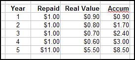
Suppose I borrow $10, to be repaid after five years pass, with one dollar of interest paid annually, and with inflation that reduces the dollar's value by ten cents each year. The "real" value of the dollar would be:

Year 0:	$1.00
Year 1:	90 cents
Year 2:	80 cents
Year 3:	70 cents
Year 4:	60 cents
Year 5:	50 cents

In year zero, when a dollar was worth $1.00, I borrowed $10. I received the value $10.

In year one, when a dollar was worth 90 cents, I paid $1 interest. I paid a year-zero value equal to 90 cents.

In year two, when a dollar was worth 80 cents, I paid $1 interest. I paid a year-zero value equal to 80 cents. The lender has received from me a total of $1.70 of year-zero value. Here, I don't need to type it all out:

Oh look at that. Open Office doesn't like the way I shortened the word accumulation.

So in this example, the  lender is repaid $8.50 out of $10 "real" value dollars. A better way to say it may be that, when we consider principal and interest and inflation, the lender received back 85% of the value lent out.

All of this of course assumes that it is reasonable to expect to be repaid at equal value rather than an equal number of dollars. In an inflationary world, that assumption may not be reasonable.

But the minimum loss to inflation is like 30%. Isn't that high?

Think this through with me.

Graph #1: The third graph from mine of 30 March

Graph #1 takes the ratio of two versions of "Federal debt as a percent of GDP". It shows nominal (current dollar) debt as a percent of nominal GDP, relative to real (2009 dollar) debt as a percent of real GDP.

I don't know what "Federal debt as a percent of GDP" shows us. I think it shows that we're ignoring private debt. But anyway, inflation (when we have inflation) makes GDP bigger and eats away at the value of existing debt. Inflation affects both debt and GDP. But it affects them differently, because debt is a "stock" and GDP is a "flow". So I have been looking at graphs comparing these things.

Graph #1 is one such comparison. It shows current-dollar values as a percent of 2009-dollar values. The nominal values vary from a low of 40% to a high around 70% of the inflation-adjusted values. Basically, it shows that creditors lost out to inflation until around 1980, and then things turned more in their favor.

Still with me?

Graph #1 only shows the value of the principal on loan. It shows some loss to creditors due to inflation, even when inflation is minimal. I think that's because, well, a 10-year Treasury note has to cope with ten years of inflation, not just one year.

Graph #2: Percent Change in the GDP Deflator from year ago (blue) and 10 years ago (red)

Two percent inflation per year is more than 20% inflation in ten years. That much inflation would knock more than 20% off the value of principle on loan. So the value of money lent would fall to maybe 75% of its initial value after a decade of 2% inflation. Graph #1 is in that ballpark.


Next: Working interest into the mix

And don't forget...

An advantage of investing in 10-year Treasury notes, and other federal government securities, is that the interest payments are exempt from state and local income tax.

- Investopedia

So I want to say what, here? The larger the Federal debt...

The larger the Federal debt, the larger is the pool of funds that are exempt from state and local tax. This financial sector untaxable, the tax burden shifts to the productive sector.