Putting numbers on vigor (3.5: That doesn't look like vigor)

Here's a close-up of that last graph from yesterday.

Graph #1: Household Debt (blue)and Trends since 2010 (dotted) and 2013 (black)

Looking at the path of household debt after the crisis. The dotted line is based on debt data from the start of the red line to the end of the green line: data since 2010. The solid black line  is based on data shown in green: data since 2013.

Just to be clear, the dotted line uses all the data that the solid black line uses, plus some earlier data. And the dotted line goes up faster.

In the years of prediction, after the green line ends, the dotted line goes up faster than the solid. The trend based on 2010-2016 goes up faster than the trend based on 2013-2016. It looks to me like the change was more rapid in the early years, less rapid in the later years. There was more vigor in the 2010-2013 decline than in the 2013-2016 increase.

It looks to me also that the increase in household debt is not as rapid as the decline in household debt service suggests:

Graph #7: Household Debt Service and the 2014-2015 Trend

But even with debt service, I now see that the 2008-2012 decline was more rapid than the the trend based on the last two years. The changes are slower now, at the bottom, than they were during the decline. Unfortunately, this is the time we should start to see increase. If the changes are slow during the time of increase, that doesn't bode well for vigor.

I do still think people are tired of this tired economy. People are ready for a better economy. And once people feel better about things, after the election maybe, household borrowing and economic vigor will rise.

// the Excel file

Putting numbers on vigor (#3: Choosing Trends for CMDEBT)

Let me ask you something: Do you think you could make a pretty good guess about the future path of this graph?

Graph #1: Household Debt Service relative to Household Debt

I can: straight line, almost flat, forever. Now... invert the ratio and look again:

Graph #2: Household Debt relative to Household Debt Service Payments

I'd guess an ever-gentler curve, always rising, but always rising less than before. That's how I imagine it. But I put a trend line on it, on the concave-down part since 2002, and the thing peaks around 2020. Peaks and starts to fall:

Graph #3: Household Debt relative to Debt Service & 2002Q1-2016Q1 Trend

I have trouble picturing it. The fall doesn't seem realistic. What to do: Go with the meticulous calculation, or the gut feel?

I decided to take another look:

Graph #4: Household Debt relative to Debt Service & 2013Q1-2016Q1 Trend

It still peaks around 2020. But when I look at Graph #1 or #2 I just don't see that kind of change happening in the next few years.

Now this is more like what I had in mind:

Graph #5: Debt Service relative to Household Debt & Power Trend since 2010Q1

Changed from the Graph #2 ratio to the Graph #1 ratio and changed the trendline type from "polynomial" to "power". I don't know if this represents the true course of future events but it does represent my gut feel.

I think I'll go with Graph #4 and Graph #5, both of them, and compare the results when I'm done. I'll predict data out to 2025 for both ratios, then factor debt service out of the ratio. That will leave me with numbers for future household debt.

Come to think of it, I can take the household debt numbers and put a trend on them directly:

Graph #6: Household Debt in billions, with Trends Since 2010 and Since 2013

Yeah. I can use the trends from Graphs #4 and #5 to predict the relation between household debt and debt service, and pull out debt in billions from those relations. Then I can compare those two outcomes to the trends on Graph #6 and see if anything at all looks copacetic.

// the Excel file

Putting numbers on vigor (#2: Projecting debt service)

Just at the end of August, at the end of my month-long investigation of debt service, FRED updated the data series. We looked at it. They added the data for 2016 Q1, and not much else changed.

I finished the "bowl" again, using the update.

Graph #1: Household Debt Service as a Percent of DPI, with projection thru 2025

Excel's second order polynomial makes a nice bowl shape. The other trendline options give a straight line or a sagging line or a line that goes off in a direction that doesn't seem right. The second order polynomial feels right. But it's a weird combination of meticulous calculation and gut feel that determines how the prediction turns out.


The trendline equation doesn't know about changes that might arise in the economy that could send the projection off in a different direction. That smooth red curve on Graph #1 will continue as far into the future as I am willing to show it. That's obviously not realistic. The trend will break eventually.

This is like the St. Louis Fed's New Characterization of the economic outlook, by James Bullard and others. They write

The concept of a single, long-run steady state to which the economy is converging is abandoned, and is replaced by a set of possible regimes that the economy may visit.

They are saying they don't know about the future, and they are now only predicting the next 2.5 years. Because they expect that trends could change.

So don't read too much into that long red line. At some point, the trend will break for sure. Maybe we'll go looking for that break point in a later part of this series.


Looking at Graph #1, the bowl seems a little lopsided. It's a little wider on the right, the red side. Between 2008 and 2012 the fall was fast. The increase after 2016 seems slower. Just by eye. Maybe that makes sense: People were faster to get rid of debt than they are to take on new debt. That could influence the debt service graph.

But the situation was different in the 1990s. That bowl looks to me to be a little wider on the left. People were reducing debt (and debt service) at a leisurely rate on the downslope of the bowl. But on the upslope, the change was less leisurely. People were excited about the economy picking up, maybe.

I think that's the case now, too. People have been hesitating, and that made for a pretty good lag. It seems like the whole of President Obama's second term was lag. But people are itching now, itching for better times. And I think people are going to start spending more, which will create the better times we're itching for. And if that happens, debt service will go up faster than Graph #1 shows.


This slower increase after 2016 on the graph, this is new. I didn't really notice it before, not in Graph #7 of the 21st, and not in Graph #3 of the 27th.

Now that I look, maybe it is there. For a better look, I put all three projections together on one graph:

Graph #2: Three Estimates of Future Debt Service

Nah, the first two run close. This new projection is a lot slower to increase.

Now I'm wondering why.

The new one, green on Graph #2, uses data from after the update. We looked at that, and there was not much changed. They just added the one data point for 2016 Q1.

That new data point was lower than the one before it. Maybe that threw the trend off? I don't know. Here is the graph that shows both versions of the data series:

Graph #3: Household Debt Service before (blue) and after (red) the update

As I said before, the new data value is down slightly from the previous number, and not much else is different.

Think that one extra data point, being low like that, could have thrown off the trend line so much?

Graph #4: Four Estimates of Future Debt Service

Yup. Graph #4 is a copy of Graph #2 but with the black line added. The black line uses the same recently-revised data as the green line, except I eliminated the data item they added for 2016 Q1.

So the difference between the green and black lines is entirely due to the 2016 Q1 item being "down slightly" from the previous number. Wow.


// the Excel file

Putting numbers on a prediction of vigor (intro)

We spent most of last month looking at household debt service, the TDSP series at FRED. Since the last recession, debt service has been showing a "bowl" shape, the left part of a bowl shape. I got all hot and bothered about the bowl. So I continued the debt service line upward to the right to complete the bowl, in the process predicting the future path of debt service.

Just so you know I'm not completely crazy, let me remind you that I also said this bowl-shape is similar to the bowl-shape you can see in the debt service numbers between 1991 and 1995. I pointed out that the earlier bowl-shape immediately preceded the good years of the latter 1990s, years the economist Robert J. Gordon called a macroeconomic miracle and that others have called "the Goldilocks years" and "the new economy". I said I expect the economy to get good again soon, as it got good during and after the "upward to the right" years of the 1990s bowl. I even said I expect labor productivity to get good again.

Maybe I am completely crazy.

Anyway, I didn't just eyeball the debt service trend. I used Excel and got a prediction in numbers. More recently, just looking at graphs, I happened to look at household debt relative to debt service. It shows a big, sweeping, upward curve. But the increase does appear to be slowing: the curve is concave-down since about 2002. I thought Oh, I can see where this line is going. I could make a guess about the future path of household debt relative to debt service.

I already have a prediction for debt service. If I can also get a prediction for the "household debt to debt service" ratio, then I can come up with a prediction for household debt in billions.

That's big. Because if I can predict the path of household debt, I think I can predict GDP and we can talk about vigor.

Well... it would be a prediction based on other predictions that essentially emerged from extending two or three lines out into the future. That doesn't seem to merit being called a prediction of GDP. Okay. But I can guess where GDP will go over the next few years, and I can put some numbers on it.

After that, instead of simply saying "I expect vigor" I will be able to tell you how much vigor I expect and when I expect it. It's the kind of prediction we can look at later and say "Art was wrong" or "Art was right". And either way, that would be a satisfying conclusion to this month-long story.


I have to break this thing up into several posts. I'd love to do it all at once. But I think each piece of it could take a couple days or more to get right.

And you should know, there is no GDP prediction till the end. I can't tell you now how things are going to turn out, because I have not done the work yet. I'd love to say there is a big prize at the end, but we won't know till we get there.

You'd think being able to say "Art was right" would be a big prize. Yeah, it would be. But we're not that far along. The last number I'll get is the GDP number. And when we look at it, we will be able to say nothing more than whether the number is reasonable.

After that, we get to wait and see how good my guess turns out to be.

The Private-to-Public (P2P) Debt Ratio in an Earlier Time

From 1920 to 1928, private debt grew at an average rate of 5.4% per year. Public debt was not growing.

In 1929, the year the Depression started, private debt growth fell to 3.7 percent. The next year it went negative. From 1931 to 1933, private debt "grew" at the rate of -7.4% per year. It fell faster than it had grown in the Roaring '20s.

From 1934 to 1945, private debt grew at an average rate of zero point eight percent. Private debt was not growing.

Graph #1: Annual Growth Rates of Public (red) and Private (blue) Debt, 1920-1950

Public debt grew rapidly in the early 1930s, offsetting the large negatives of private debt. Public debt grew slowly in the latter 1930s, after the collapse of private debt had been halted. Public debt spiked during World War Two.

The growth of private and public debt shown on Graph #1 affected totals in both categories and moved the P2P ratio:

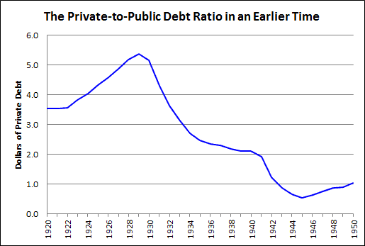
Graph #2: Private Debt relative to Public Debt, 1920-1950

The P2P ratio peaked in 1929 at $5.40 private debt for every dollar of public debt. Then it fell -- rapidly at first, because of the rapid negative growth of private debt and the rapid increase in public debt. But after policymakers slowed the decline of private debt, the growth of public debt was reduced. And as a result, Graph #2 shows a definite slowing of the downtrend between 1934 and 1941.

The slowing of the downtrend extended the time it took to to bring the ratio low enough that the economy could resume growth.


It is foolish policy that allows the P2P ratio to reach such high levels. But only a fool would say that a Great Depression is the right solution to those high levels.

Nor is it the right solution to prevent the collapse of private debt, for this only pushes the good years farther off into the future.

The best solution is to prevent the ratio from climbing to such high levels. Prevent it before it happens. This means that policymakers must stop the growth of private debt before it creates a crisis.

You might think there are two ways to reduce the Private-to-Public debt ratio: Either reduce the growth of private debt or increase the growth of public debt. But increasing the growth of public debt turns out to be ineffective. Stuff happens: In the mid-30s the growth of public debt was reduced. In the 1970s and '80s the rapid growth of public debt induced rapid private debt growth, keeping the ratio at a high level for many years. And in recent years, policymakers have held that public debt growth must be restrained.

So there is really only one way to reduce the ratio of private-to-public debt, and that is to reduce private debt.

Public Debt Cannot "Get Ahead" of Private Debt

Download as PDF

In a recent note on the concern over public debt, Lars P. Syll points out that the focus “is solely on the upper limit of indebtedness”. Syll says there may also be a problem “if public debt becomes too low” or “too small.”

Public debt, however, is not too small. At least, not in the United States:

Figure 1: Showing the Growth of the Federal Debt above and beyond its pre-1975 Trend

If the 1945-1974 trend of Federal debt growth had continued unchanged to 2015, we would have ended up with a one-trillion-dollar debt. Instead, we got $18 trillion. The problem is surely not that the Federal debt is too low or too small.


Syll considers balanced budgets (“People ... are as a rule worried and negative” about “public sector budget deficits and debts”) and Ricardian equivalence (“financing government expenditures through taxes or debts is equivalent”). He contrasts the “rather widespread consensus” (“public debt [is] acceptable as long as it doesn’t increase too much and too fast”) with the view of “both Keynes and [Abba] Lerner” (“Public debt is … a means to achieving two over-arching macroeconomic goals – full employment and price stability”).

Syll has the consensus saying a high level of public debt hinders growth. He has Wolfgang Streeck saying just the opposite: slow growth caused the increase in public debt. Despite the difference of opinion, there seems to be agreement that GDP is the right context to use.

But GDP is not always the best context for debt. For if the economy slows, there is less GDP but no less debt. Then too, one needs money to pay down debt, but money is destroyed when debt is repaid. GDP is important -- income is important -- because it brings us money. But we pay down debt with money, not with GDP.

There is another, better context for debt. Lars Syll comes close to identifying it when he writes: “Central to the Keynesian influenced view is the fundamental difference between private and public debt.” But Syll fails to pursue that fundamental difference.

The better context for debt is debt: Public debt relative to private, or private relative to public. Consider the relation between private and public debt:

Figure 2: Non-Federal Debt relative to the Federal Debt

While the economy was good in the 1950s and '60s, the line was going up. While the economy was good in the latter '90s, the line was going up.

When the line is trending down, as from 1974 to 1993, the economy is preparing to have the line go up again later. It is preparation for good times to come. When the line is falling more severely, as in the years since 2008, it is again preparing for good times to come.

Low and rising is good. High is not so good. Falling is preparation.

Why was the increase from the early 1950s to 1974 on Figure 2 so much more rapid than the decline from 1974 to 1993? Come to think of it, why was the decline of 2008-2016 so much more rapid than the decline from 1974 to 1993?

The latter question is easy to answer: There was no “panic” in 1974. The panic of 2008 sent the debt ratio tumbling, with private sector debt deleveraging combined with massive public deficits. We saw nothing like that in the 1970s.

In the 1970s, “safety net” policies put in place during and after the Great Depression accelerated the growth of public debt. This reduced the debt ratio. But the private sector was not in the midst of deleveraging. Private debt grew rapidly on the enlarged foundation of public debt. Private debt in those years grew almost as fast as public debt. Because private debt growth was hindered by neither crisis nor policy, it took 19 years to bring the ratio down enough that the economy could again grow with vigor.

In the 19 years before 1974, when the economy was good, private debt grew nine times faster than public debt. That’s why, after 1974, the economy needed rebalancing.

In the 19 years from 1974 to 1993, Federal grew more than 13 times as fast as in the 19 years leading up to 1974. But private debt grew nearly as fast as public debt, so the debt ratio came down only slowly.

The problem in the years of rebalancing was not that public debt was "too low" as Syll might suggest. Rather, the problem was that the debt ratio could not easily fall while private debt growth continued at such a rapid pace. The problem was not that public debt growth was too low, but that private debt growth was too high in a time when rebalancing was required.

The public debt is too small? I don't think so.

If the 1945-1974 trend of Federal debt growth had continued out to 2015, we would have ended up with a one trillion dollar debt. Instead, we got $18 trillion:

Graph #1: Showing the Growth of the Federal Debt above and beyond its pre-1975 Trend

How does he miss it?

Lars P. Syll:

Today there seems to be a rather widespread consensus of public debt being acceptable as long as it doesn’t increase too much and too fast. If the public debt-GDP ratio becomes higher than X % the likelihood of debt crisis and/or lower growth increases.

But in discussing within which margins public debt is feasible, the focus, however, is solely on the upper limit of indebtedness, and very few asks the question if maybe there is also a problem if public debt becomes too low.

The government’s ability to conduct an “optimal” public debt policy may be negatively affected if public debt becomes too small.

That's downright funny: The focus is solely on the upper limit of indebtedness.


I keep coming back to read Syll's post again and again. This is the third time I've started a response to it. The others didn't make it.

Here's my problem with Syll's statement: He considers "public sector budget deficits and debts" and says that many people "raise their voices to urge for reducing the debt". But his reply to those people is that the public debt may be "too low" and "too small".

People say the public debt is too big, and Syll says it's too small. It is a disturbingly empty rebuttal; if it isn't funny, it isn't anything at all.


One of the things that bothers me about Syll's post is that I could follow his whole argument right up to the end, and then it all fell apart in the last paragraph. Syll writes:

To guarantee a well-functioning secondary market in bonds it is essential that the government has access to a functioning market. If turnover and liquidity in the secondary market becomes too small, increased volatility and uncertainty will in the long run lead to an increase in borrowing costs. Ultimately there’s even a risk that market makers would disappear, leaving bond market trading to be operated solely through brokered deals. As a kind of precautionary measure against this eventuality it may be argued – especially in times of financial turmoil and crises — that it is necessary to increase government borrowing and debt to ensure – in a longer run – good borrowing preparedness and a sustained (government) bond market.

I understood every word for 26 paragraphs. Then in the 27th, Syll collapsed into economist-speak.

Syll seems to be saying that a "well-functioning secondary market in bonds" is good for the economy. I guess I can agree with that.

The rest of the paragraph is all speculation. Syll suggests that we need might more bonds to keep the market well-functioning -- "especially in times of financial turmoil and crises". This seems to be a rewording of the old post-crisis argument that there was a shortage of safe assets.

Seems to me to be too much focus on finance, not enough focus on the real sector, and not enough focus on the cost finance imposes on the real sector.


Disputing the argument that public debt is too big, Syll takes the evaluation and stands it on its head: He says public debt is too small. It irks me no end. I would take the focus of the argument -- public debt -- and stand that on its head instead.

I would say private debt is too big.

She smiles

I like Michael Hudson. I think he's interesting. Dirk Bezemer too. I agree with a lot of what these guys say. But if I agreed with everything they say, then I would have no need to write -- no need to point out things that smell fishy.

So... as Tom Mathias says to Mared Rhys: "You ready?"


Bezemer & Hudson: Finance is not the economy: Reviving the conceptual distinction. A damn long article.

From the Abstract:

Conflation of real capital with finance capital is at the heart of current misunderstandings of economic crisis and recession. We ground this distinction in the classical analysis of rent and the difference between productive and unproductive credit. We then apply it to current conditions, in which household credit — especially mortgage credit — is the premier form of unproductive credit.

So it's my fault, is it? I bought a house. By definition -- by their definition, not mine -- that was "unproductive".

I have trouble with their story already, and I didn't even get out of the Abstract.

It's a dangerous thing when one group of people points to another group of people and says those are the bad people. Economic activity requires cooperation.


"How did we get so indebted," they ask, "without real wage and living standards rising, while cities, states, and entire nations are falling into default?"

Good question. My answer is simple: Economic policy encourages credit use and discourages the repayment of debt. That's how we got so indebted.

Bezemer and Hudson's answer is less Occam than mine:

The last quarter century’s macro-monetary management, and the theory and ideology that underpinned it, was lauded by leading macroeconomists ... Oliver Blanchard, Ben Bernanke, Gordon Brown, and others credited their own monetary policies for the remarkably low inflation and stable growth ... But it was precisely this period from the mid-1980s to 2007 that saw the fastest and most corrosive inflation in real estate, stocks, and bonds since World War II.

Nearly all this asset-price inflation was debt-leveraged. Money and credit were not spent on tangible capital investment to produce goods and non-financial services, and did not raise wage levels.

There ya go: unproductive debt. It comes with a story, but the moral of their story is "unproductive debt".


"This financial expansion," they write,

This financial expansion took the form more of rent extraction than of profits on production (Bezemer and Hudson 2012) — a fact missed in most analyses today (for a proposal, see Kanbur and Stiglitz 2015). This blind spot results from the fact that balance sheets, credit, and debt are missing from today’s models.

Well, far as I'm concerned, they are right but they quickly lose focus. "... a fact missed in most analyses today." Irrelevant. "This blind spot results from the fact that balance sheets, credit, and debt are missing from today’s models." Beyond irrelevant.

The trick is to simplify, not amplify.

"This financial expansion took the form more of rent extraction than of profits on production". Yeah, I know. I looked at that. (Time to update that old post. None of the graphs seem to work now.) The way I figured it, if you take the financial profits of nonfinancial corporations and put them with the profits of financial corporations, you get about $3 in financial profit for every dollar of profit on production. That's not good.

But I don't know why they call it "rent". The payment to finance is interest.


Bezemer and Hudson:

To explain how the bubble economy’s debt creation leads to debt deflation, we distinguish between two sets of dynamics: current production and consumption (GDP), and the Finance, Insurance and Real Estate (FIRE) sector.

Yup. But

It is as if there are “two economies,” which are usually conflated. They must be analyzed as separate but interacting systems, with real estate assets and household mortgage debt at the center of the bubble economy.

There it is again. See it? They are saying: You, it's you people with mortgages that are the problem... And you other guys, who want mortgages, you're part of the problem.

That's not how I see it. As I see it, policy is the problem.

In section three, therefore, we examine the significance of household debt. In today’s “rentier economy” this represents not real wealth, but a debt overhead.

Maybe. Maybe household debt has different "significance" in "today's 'rentier economy'" than it did in the economy before the 1980s. I don't know about the "significance" of debt. I focus on the cost of debt.

In section four, we discuss the pathologies arising from this overhead: loss of productivity and investment, with rising inequality and volatility.

And now we arrive at the crux of the matter. In section four, Bezemer and Hudson discuss the problems arising from the "debt overhead". But don't we know about that already?

People who already know debt is a problem already know about about "pathologies" arising from excessive debt. We don't need schooling in that. We need to talk about how we got into the mess. Because you're not going to be able to get out of the mess unless you know how you got into it. I mean, for example, if Bezemer and Hudson do not realize that the growth and excessive accumulation of debt was a direct result of policies that favor credit use and debt maintenance, then they are not likely to reach conclusions that call for a change in those policies.

Simplify.


In Hinterland, on Nexflix, s2e3, near the end, they've wrapped things up and they're ready to leave the scene. DCI Mathias walks over to the car, opens the door, looks at DI Rhys and says, "You ready?"

She smiles, just the slightest smile.